Reconstructing leaf growth based on non-destructive digitizing and low-parametric shape evolution for plant modelling over a growth cycle
Henke M., Huckemann S., Kurth W., Sloboda B. (2014). Reconstructing leaf growth based on non-destructive digitizing and low-parametric shape evolution for plant modelling over a growth cycle. Silva Fennica vol. 48 no. 2 article id 1019. https://doi.org/10.14214/sf.1019
Highlights
- A complete pipeline for plant organ modelling (at the example of poplar leaves) is presented, from non-destructive data acquisition, over automated data extraction, to growth and shape modelling
- Leaf contour models are compared
- Resulting “organ” modules are ready for use in FSPMs.
Abstract
A simple and efficient photometric methodology is presented, covering all steps from field data acquisition to binarization and allowing for leaf contour modelling. This method comprises the modelling of area and size (correlated and modelled with a Chapman-Richards growth function, using final length as one parameter), and four shape descriptors, from which the entire contour can be reconstructed rather well using a specific spline methodology. As an improvement of this contour modelling method, a set of parameterized polynomials was used. To model the temporal kinetics of the shape, geodesics in shape spaces were employed. Finally it is shown how this methodology is integrated into the 3D modelling platform GroIMP.
Keywords
growth modelling;
non-destructive data acquisition;
automated data extraction;
image processing tool;
leaf shape modelling;
reusable modules;
Populus x canadensis
-
Henke,
Department Ecoinformatics, Biometrics & Forest Growth, University of Göttingen, 37077 Göttingen, Germany
E-mail
mhenke@uni-goettingen.de

- Huckemann, Institute of Mathematical Stochastics, University of Göttingen, 37077 Göttingen, Germany E-mail huckeman@math.uni-goettingen.de
- Kurth, Department Ecoinformatics, Biometrics & Forest Growth, University of Göttingen, 37077 Göttingen, Germany E-mail wk@informatik.uni-goettingen.de
- Sloboda, Department Ecoinformatics, Biometrics & Forest Growth, University of Göttingen, 37077 Göttingen, Germany E-mail bslobod@web.de
Received 15 October 2013 Accepted 12 March 2014 Published 20 May 2014
Views 479960
Available at https://doi.org/10.14214/sf.1019 | Download PDF

List of symbols
| Abbreviation | Unit | Description |
| Plant material | ||
| T1 | - | Set of leaves taken from tree one |
| T2 | - | Set of leaves taken from tree two |
| T3 | - | Set of leaves taken from tree three |
| T1–3 | - | T1∪T2∪T3 |
| t | d | Time |
| Size model | ||
| l0 | m | Initial leaf length on its first day of measurement (t = 0) |
| m | - | Parameter of the leaf length function |
| k | - | Parameter of the leaf length function |
| n | - | Parameter of the leaf length function |
| Proportional shape model | ||
| l | m | Maximal leaf blade length |
| bl | m | Maximal width of left half of leaf blade |
| br | m | Maximal width of right half of leaf blade |
| lml | m | Normalized position on the midrib where the maximal left width is attained |
| lmr | m | Normalized position on the midrib where the maximal right width is attained |
| bl / l | - | Shape parameter; ratio between maximal left width and length |
| br / l | - | Shape parameter; ratio between maximal right width and length |
| lml / l | - | Shape parameter; ratio between lml and length |
| lmr / l | - | Shape parameter; ratio between lmr and length |
| Geodesic model | ||
| x(t) | Modelled configuration landmark matrix at time t | |
1 Introduction
1.1 Motivation
Realistic modelling of plant growth is one of the key issues in ecoinformatics. In plant modelling, structural elements such as leaves play an essential role (Lecoustre et al. 1992; Prusinkiewicz et al. 1994). They are the main interface between the plant and its environment. Furthermore, they determine radiation interception and, thus, gas exchange and photosynthesis, which are the main factors of growth. Various functional-structural plant models (FSPMs) using several different software systems, e.g. GroIMP (Kurth 2007; Kniemeyer 2008; GroIMP Developer Group 2013), GreenLab (de Reffye et al. 1997; Hu et al. 2003), LIGNUM (Perttunen et al. 1996), AMAPStudio (Griffon and de Coligny 2012), LStudio (Biological Modeling and Visualization research group 2013) and Almis (Eschenbach 2000) have been developed for these issues.
Crop models are a common tool for estimating yield or biomass development in agri-, horti- and silviculture (Ruiz-Ramos and Mínguez 2006). However, classical crop models do not take into account plant architecture, let alone the growth of a single leaf. Plant structure gets into the focus in the development of new 3D crop models. Studies on leaf area already have a long history, going back to the beginning of the 20th century (Gregory 1921). Measurements were done manually (Gallagher 1979) for winter wheat and spring barley, and even recently, Chen et al. (2009) measured leaf lengths for over 1700 hours with a ruler, which is often the common way of obtaining data. Even when technical help was used for digitisation, the image segmentation was still done manually, e.g., Neto et al. (2006) extracted 510 leaves by hand. In order to obtain statistically meaningful results, a large number of measurements has to be done, which requires large human and financial resources.
1.2 Objectives and goals
The aim of this research is to provide:
- a simple, effective, non-destructive and field-applicable method to acquire forms of leaves during a growth cycle,
- an image processing tool to automatically extract leaf data from a large number of images,
- a model for leaf shape development that is parsimonious with respect to the number of parameters yet as realistic as possible, and,
- an integration of this model into an existing software environment allowing for rule-based (Kniemeyer 2004) realistic plant modelling.
In order to accomplish aim (a), we used a photogrammetric device consisting of a digital reflex camera within a rigid frame providing high accuracy of measurement while keeping every investigated leaf completely intact for frequently repeated measurements over its entire growth period. During such measurements, each leaf is measured / photographed several times. This has to be done for several leaves in order to obtain a statistically significant database, resulting in some hundred images, which need to be automatically extracted in a reproducible way. Thus, an ImageJ (ImageJ Developer Group 2013) macro as image processing tool (b) was developed and used. Concerning (c), reducing the number of parameters decreases the accuracy of the model, calling for search of a good trade-off. We propose to model the leaf forms with polynomials determined by a minimal set of 5 to 13 real-valued parameters. The set of these parameters defines form as size and shape in an abstract shape space. Fig. 1 illustrates all the phases of the workflow beginning with data collection, interpretation, representation and ending at the integration of the resulting model within new or existing FSPMs.

Fig. 1. Overview of the described workflow: showing the steps from photographing leaves to the integration of the resulting organ modules into an existing FSPM.
During the proof of concept phase, it turned out that the investigated leaves can be accurately modelled with the few parameters proposed. In the final step (d), the developed leaf models are implemented in the eXtended L-System modelling language (XL) (Kniemeyer 2004, 2008), a programming language created specifically for use in functional-structural plant modelling (Kniemeyer et al. 2007). It is an extension of Java that combines the advantages of an imperative and object-oriented language with those of a rule-based rewriting language. We use the modelling software GroIMP (Kurth et al. 2006; Kurth 2007; GroIMP Developer Group 2013) for implementation. Thus, the leaf components based on the above models are available for use in XL in different functional-structural models. These new plant organ modules facilitate the building of realistic complex models as they just need to be used and parameterized without the need to care about any implementation details.
1.3 Previous work
As far as we know, the task we set has not been tackled as a whole, while there is vast literature for several of these components, e.g., Dornbusch and Andrieu (2010) introduced the Lamina2Shape program, which was written in the commercial software MATLAB (The MathWorks, Inc.). They propose cutting the leaves and using a flatbed scanner for image acquisition. Using a scanner, of course, makes it impossible to observe growth of one individual leaf over the whole growth period which is often desirable (Maksymowych et al. 1973). This is particularly important when different temperature treatments influence leaf growth and, consequently, the total biomass production (Peacock 1975; Dennett et al. 1978). Use of commercially available leaf area meters (like the LI-3100, LI-COR Inc., Lincoln, Nebraska, USA) is another common destructive way of measuring leaf area (Routhier and Lapointe 2002; Reich et al. 2004).
These methods cannot be used to acquire data of an individual leaf over the whole growth cycle, which is a major limitation for the use in several FSPMs that have the aim to reproduce the dynamics of growth and morphological development in realistic detail. Further, most of these methods cannot be applied in the field, which restricts the number of species that can be investigated.
Electromagnetic 3D digitizers (e.g. Fastrak, Polhemus, USA) that are also used for digitisation of leaves (Wiechers et al. 2011) have several restrictions, too. First, it is difficult to avoid influencing the measurements by, e.g., touching the leaves while still aiming to be as close as possible in order to obtain correct data, and to avoid wind and breathing effects. Second, several points need to be recorded and repeatedly measured for each leaf. Thus, each point needs to be touched over and over again, so that marks on the leaf would be needed, which could alter leaf development. Apart from that, a thigmomorphogenesis (stunted growth due to touching) effect might ensue from repeated probing by the stylus and the hand of the digitizing person.
Regarding leaf growth models, several methods have been proposed in the literature. The most common way is to separate shape and size and model both aspects independently (Mosimann 1970). Functions or curves are used to generate a contour in most models in order to describe the shape (Chi et al. 2003; Dornbusch et al. 2011). State variables such as leaf length, leaf area or dry weight will change with time and are thus usually described using a growth function of time (e.g., Gompertz, logistic, Richards, Weibull, the beta growth function, or spline functions (Richards 1959; Richards 1969; Yin et al. 2003)). Note that there is usually no statistically significant difference between the fitted Richards curves and the Gompertz curve (Hackett and Rawson 1974).
Statistical methods have also been applied to model shape: Neto et al. (2006) used a chain encoded leaf contour as a basis for an elliptic Fourier descriptor. In this way (and using principle component analysis) they described the leaf shape, in order to reduce the total number of Fourier coefficients from 4h − 3 (with h = 30 being the harmonic number). However, this method is still not practically applicable in an FSPM, as trees have hundreds or thousands of leaves of different ages. Finally, Chien and Lin (2005) used elliptic Hough transformations for shape description.
2 A simple and efficient photometric method
2.1 Recording equipment
In order to acquire realistic growth data from biological objects at hand, the method to be employed needs to be accurate, reliable, robust, and easily operable in field use under natural lighting conditions; non-destructive and not affecting natural growth since we want to frequently assess each object over a longer period of time at regular intervals. In particular, any impacts on natural growth during the data collection need to be minimized in order not to falsify the original data.
The framework presented here uses a digital reflex camera, Sigma SD9 with a Sigma 50 mm macro-objective (SIGMA Deutschland, Rödermark, Germany). The full image resolution of 2268 × 1512 pixels was used, which translated into 14.58 pixels per mm. As an advantage, the Sigma camera model features a Foveon X3 image sensor, which uses an array of photosites: These consist of three vertically stacked photodiodes for the three main colours (red, green, and blue), instead of arranging them next to each other, as is the state-of-the-art of common CMOS-sensors and which would always induce a slight measurement bias. Other types of camera equipment with appropriate resolution are suitable as well. For the photographs the camera is fixed on a rigid device by means of a threaded bush that otherwise is used to fixture a tripod. The device consists of a rectangular rigid frame with an attached screen on the front (covered with a glass pane) for fixing leaves (Fig. 2). The windowpane uses an antireflection coated glass. This simple but robust construction is easy to use and comparatively cheap.
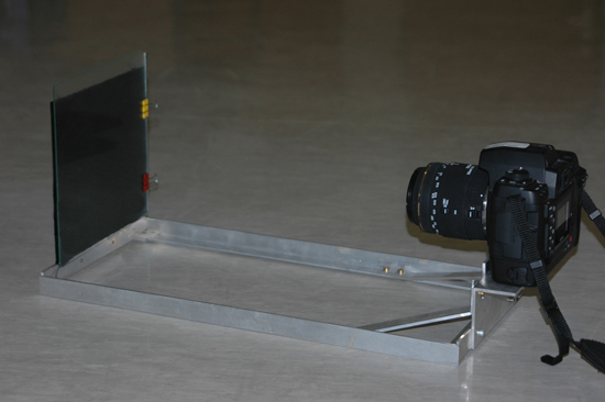
Fig. 2. Recording equipment. The use of an additional black board to cover the shining metal arms is recommended in order to prevent reflections, as well as the use of a second carrying strap fixed near the object plane to prevent toppling and to improve equilibrium for field use.
An advantage of the quite inflexible construction is that the object plane is oriented parallel to the projection screen so that perspective distortions are nearly completely eliminated. In effect, the pictures extracted do not have to be equalized. The fixed distance as well as the fixed focal length allow for the use of a reproduction scale constant over the entire data extraction process. In particular there is no need for recalibration or rescaling for each image taken. Because of the usage of a macro lens there is no need for any correction of optical aberrations: the latter could be necessary when a normal lens is used at a relatively short distance such as the one between the object plane and the projection screen.
Black cotton velvet serves as background (Fig. 3b). On the one hand its soft and flexible tissue helps to avoid damage to the 3D structure of the leaf and lets it sink in smoothly while it is fixed non-destructively. On the other hand it absorbs nearly hundred per cent of the shadows cast by the leaf’s 3D structure (Fig. 3a), which are not negligible despite their small size. Without the velvet these shadows cast by the leaf would have to be corrected for in a laborious pre-processing step. Alternatively, in order to avoid shadows altogether the leaf contour would have to be fixed to the background, thereby possibly harming the protruding leaf veins. Since the scaling factor of our measuring apparatus was determined prior to data acquisition, the true size of leaves photographed in front of the velvet background can be easily determined.

Fig. 3. Edge effects of different backgrounds. a) The photograph clearly shows a wide shadow that would cause problems in case of an automatic segmentation. b) A black velvet as background absorbs nearly all shadows and provides a soft structure allowing the leaf to sink in.
2.2 The image processing tool
Of the images mentioned in the previous chapter, only the 2D contours bounding the leaves are of interest for the present application. Ultimately we would like to obtain from every acquired image a list of coordinate pairs (x, y) describing this contour (Fig. 4). Extracting contours is a typical image processing challenge which can be met by a variety of well-developed tools. Due to our specific recording equipment, the images are well prepared for this task as they are basically black (velvet) and green (leaf blade). When splitting the original image into its red-green-blue colour channels, only the green channel is used for further processing. This channel provides the highest contrast for the picture and facilitates segmentation, which in turn is realized by iterative adaptive thresholding. In the ensuing steps the picture is clipped, the background is cleared up and holes in the leaf if any are closed. In the next step the leaf petiole is removed from the obtained contour. Subsequently the leaf is rotated until its top and petiole entry point are aligned vertically. The resulting contour is stored as a list of 200 to 2500 coordinate pairs, depending on the size of the leaf, converted into mm with the leaf-base moved to the origin of the Cartesian coordinate system. As additional output values, maximum length, width and leaf area are obtained for each leaf.
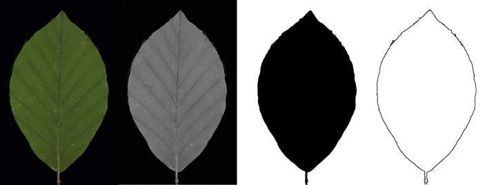
Fig. 4. Schematic workflow of contour extraction: Original image (colour picture) / green channel (grey-value image) / threshold image (black-white picture) / contour picture.
The process described here was compiled as an image processing tool and implemented as an ImageJ macro (ImageJ Developer Group 2013). It permits the handling of complete directories into which all contours of collected images are extracted automatically as data files. However, two manual inputs are recommended: First of all, the user may opt for manual correction of an automatically determined threshold value, e.g. if a photograph was taken under unfavourable lighting conditions or if the ratio between leaf area and background is too variable, e.g., in the case of very big or very small leaves (as the automatic threshold finding is calibrated for medium-size leaves). Secondly, the user may want to specify the point at which the petiole is joined to the leaf blade. While this location can be automatically detected for most leaves, e.g. for all those depicted here, some petioles are running parallel to the base of the leaf blade or even pass in front of the leaf blade, making automatic extraction unreliable.
Bad image quality is in fact a common problem. Moreover in field use, lighting conditions are always problematic, e.g., sun reflections, shadows, blur due to wrong focus or aperture settings; illumination problems (over- and underexposure); and an exaggerated contrast. Tests and extended field use have shown that the image manipulation workflow presented here is surprisingly robust and resistant against these interferences which in a controlled laboratory environment would actually require no further attention. The script is free, open-source and available upon request from the first author.
3 Plant material
For this study, we chose three trees of the Canadian Black Poplar (Populus × canadensis Moench), each representing a different clone, from an experimental stand at the University of Göttingen, Germany (51°31´N, 09°55´E). The study was conducted in 2008 on 5-year-old trees having a height of 140 to 250 centimetres (Table 1). From each tree during the entire growth period from spring to fall, 16 leaves were selected and measured, daily in the beginning, every two to four days subsequently. Some leaves had to be replaced by new leaves during the measurement period due to damage (scratches or big holes) or natural shedding. Leaves were sampled from different canopy heights to account for within-tree height effects, which were, however, not considered in this study.
| Table 1. Summary statistics of the three trees that were used to build the data base for this study. From each tree a set of leaves was randomly chosen and observed over the whole period of growth. | ||
| Tree | Number of leaves | Number of measurements |
| T1 | 20 | 262 |
| T2 | 12 | 162 |
| T3 | 11 | 158 |
| Total | 43 | 582 |
Black poplar leaves were chosen for a number of reasons: first of all they do not resinate and are therefore not likely to soil the equipment; second, for the proposed photometric method we required flat, non-undulating leaf blades. Third, for advanced studies of inter clone differences planned in the future we needed a set of clones and a reference tree, which were only available for a limited set of species. Finally, in order to demonstrate our shape model at a simple example, a leaf with a simple contour was preferable. Leaves of, e.g., beech, birch, alder, or elm can be analysed in a similar way. For lobed leaf shapes such as maple or oak more sophisticated contour models are necessary.
In the following, the three trees are denoted by T1, T2 and T3.
4 Leaf modelling
In our approach, we will neglect microstructure growth. Within a parameterized set of forms the statistically closest match is searched for, as in landmark-based shape analysis (Dryden and Mardia 1998). This paradigm lacks a premeditated biological model; rather biological data will be naturally associated with an appropriate model from a family of generic parsimonious models.
In particular we want to describe form by a tuple of one-dimensional size and multidimensional shape. As a common assumption for biological objects, we expect that growth affects both size and shape. A factorization into size and shape is in no way canonical (e.g. Mosimann (1970) for a broad discussion).
Statistical calculations and parameter fitting were done using the R language and environment (R-Project Developer Group 2013). The analyses presented here are restricted to single leaves, time series of individual leaves, and sets of leaves of individual trees.
4.1 Size modelling
In this work, we use the distance from petiole to tip, approximating the length of the main leaf vein, as the size variable. This attribute can easily be collected and has a simple geometric meaning. Size growth (Eq. 1) in time t [d] is modelled according to the Chapman-Richards growth function (Richards 1959), a standard growth function with parameters m, k and n determined by a least-squares fitting process.
![]()
with l0 being initial leaf length at t = 0, and m + l0 the maximum possible length which is approached asymptotically. In fact, the fitted growth functions represent individual temporal leaf kinetics rather well. Fig. 5 shows a function fitted to our whole data set.
The empirical distribution of coefficients m, k and n for the three trees is displayed in Fig. 6. The model was fitted for each leaf separately. It can be seen that the overall variation of coefficients within trees is rather large. As expected, the variation of the mean or median coefficients across trees is rather small (Fig. 5).
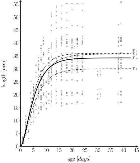
Fig. 5. Fitted length function, based on 582 measurements on a total of 43 individual leaves taken from three different trees (T1 = 262, T2 = 162, T3 = 158 measurements) over one growth period. Solid line: fitted leaf length function over whole data set (T1–3 = T1∪T2∪T3) (Eq. 1; m = 34.224 ± 0.595 (mean ± SD), k = 0.249 ± 0.027, n = 1.859 ± 0.295, l0 = 0); Dashed lines: fitted functions for each individual tree; T1 (triangles), T2 (dots) and T3 (squares): measured leaf data.
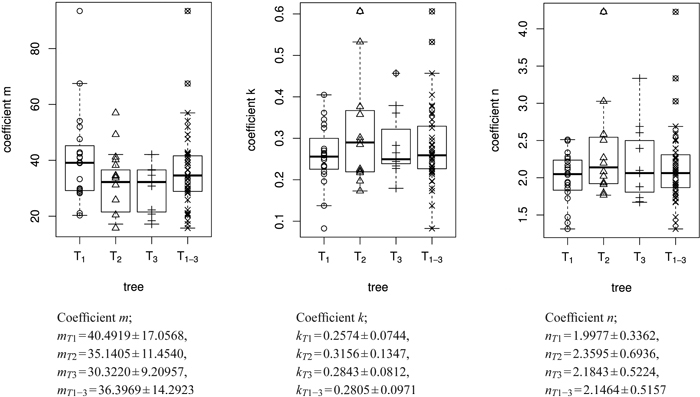
Fig. 6. Overview of the size model coefficients’ m, k and n in box and whisker plots (median, IQR, whiskers at 1.5 IQD or extremal values) broken down to the level of individual leaves (in total 43 leaves) and ordered by tree (T1, T2, T3). The fourth column in each figure illustrates the combined results of all three trees taken together (T1–3 = T1∪T2∪T3), see Table 1. Below we report the mean ± SD of the respective size model coefficients.
4.2 The proportional shape model
We begin our considerations for shape modelling with a minimal set of discriminative shape parameters (Fig. 7). Since leaf length accounts for size, clearly, maximal left and right leaf width bl and br are the first descriptors for shape. Moreover, for meaningful shape discrimination the vertical locations lml and lmr where the maximal left and right width is attained, respectively, seem essential.
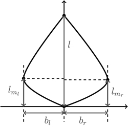
Fig. 7. Depicting the four shape parameters of the proportional model on a leaf contour. See list of symbols for further explanations.
For the leaves observed, the ratios of widths to length as well as of vertical locations to length were determined, for 83 leaves from one day of observation and for each tree separately over the growth period (see sub-figures 8a to 8c for some summaries).
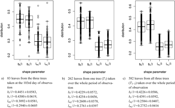
Fig. 8. Distribution of shape parameters in box and whisker plots (median, IQR, whiskers at 1.5 IQD or extremal values) of a) 83 leaves measured on one single day, b) of one tree and c) of all three trees taken together over the whole period of observation. Below we report the mean ± SD of the respective shape parameters. See list of symbols for further explanations.
Fig. 9 shows a linear regression of the shape variables to the size variable for both data sets, the one with 83 leaves from three trees taken at the 103rd day of observation (Fig. 9 a–d) and the one of 262 leaves from one tree (T1) taken over the whole period of observation (Fig. 9 e–h). For all data sets we observed nearly constant shape parameters bl / l and br / l (slightly positively correlated), as well as lml / l and lmr / l (slightly negatively correlated) showing that the vertical position where the maximal width occurs moves with age from a position around one third of the total length towards one quarter of the leaf. In conclusion, we can say that length qualifies as a fairly good predictor of shape.
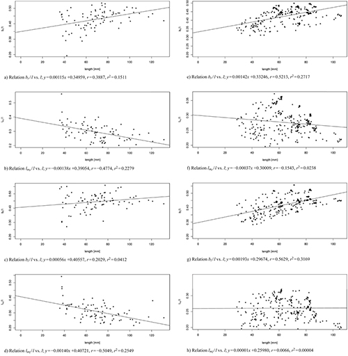
Fig. 9. Linear modelled relation between the model parameters bl / l, br / l, lml / l, lmr / l and the leaf length l of 83 leaves from three trees taken at the 103rd day of observation (sub-figures a–d) and of 262 leaves from one tree taken over the whole period of observation (sub-figures e–h). Correlation coefficient r and multiple R-squared r2. See list of symbols for further explanations. View larger in new window/tab.
4.3 Contour models
4.3.1 Spline interpolation
Here, we propose two models that allow reconstructing a realistic leaf contour from the four shape parameters and the single size parameter. In fact the first model uses only the four shape parameters of the proportional model; the second model learns its parameters from real contours.
We start with computing separate spline curves for the left and the right part of the leaf contour. More precisely, for each side, three control points S0, S1, S2 are determined (Fig. 10; for the left side which was turned counter clockwise by 90°). Note that (bl, lml) and (br, lmr) are not extreme points of the resulting spline curve. In order to make them extreme we inserted an additional point between S0 and S1 (calculated as S0b = (lml / 2, 2bl / 3) for the left side and similarly for the right side), and possibly one more close to S2, to sufficiently bend the curve downward to obtain a more globular bellied shape.
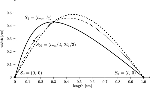
Fig. 10. Comparison of spline interpolation (dashed) between the three support points S0, S1, and S2 which overshoots the maximum width with the bi-interpolation C(s) (solid, black) interpolating splines for contour of the left side of the leaf. Additionally a spline interpolation between four support points (S0b = (lml / 2, 2bl / 3)) is included (dotted).
Alternatively, in order to guarantee that the points (bl, lml) and (br, lmr) were indeed extreme for the modelled leaf contour we calculated a parametric curve C(s) (Eq. 4), the X and Y values of which are interpolated separately by two Hermite interpolations sp1(s) and sp2(s) between temporal supporting points Tx0, Tx1, Tx2 used for sp1(s) and Ty0, Ty1, Ty2 for sp2(s), with u1 and u2 which take for the left side of the leaf contour the form
![]()
![]()
The final curve C is defined by Eq. (4), with s ∈ [0,u2]
![]()
Similarly, we proceed for the right side of the leaf contour. Fig. 11 depicts a typical leaf reconstruction by the proposed bi-interpolation of the proportional model.
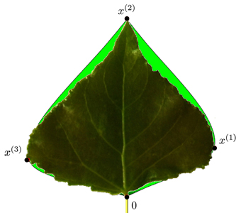
Fig. 11. Modelled contour approximation by bi-interpolation of the proportional model versus the original leaf contour. x(t) are the special contour points used in this model.
4.3.2 A general polynomial fit
Once again, we can take advantage of the fact that for the poplar leaves investigated we may model each leaf side (left and right) separately. Moreover they exhibit the favourable property that each half-contour (left and right) can be viewed as a function of vertical height. We now model each half-contour separately by a fifth degree polynomial (Eq. 5) by pointwise fitting (Fig. 12a).

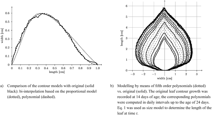
Fig. 12. Reconstruction of a leaf contour over time and comparison of the contour models with original model.
For every single leaf of a time series, meaning for every point in time ti,i ∈ [0,n], when the leaf image was captured, a tuple of coefficients ctti = (c0, c1, c2, c3, c4, c5) is fitted via least squares to the model (Eq. 5). The n + 1 coefficient tuples are combined to a coefficient matrix M:

In order to determine the coefficients at times between the moments when photos were taken, the coefficients of the same degree are spline interpolated.
As a further, optional enhancement step to model contours more realistically, another function is added to the leaf function, so that the sum will produce a slightly serrated edge, which matches the specific shape of poplar leaves quite well. As such a Fourier-series approximation of the so called saw-tooth function (Eq. 7) is used:
![]()
At this stage we use a generic function for all leaves of a species where the parameters a and b have been obtained from a fit to one representative leaf. Such a supplement might be seen at first sight only as an ‘aesthetic correction’ increasing computation time, as in the case of poplar leaves. However, applied to other species with more serrated leaf contours it will become significant for more realistic light interception and self-shading effects. Notably, the proposed saw-tooth function is a parsimonious approximation increasing the level of realism.
Fig. 12b depicts a typical reconstruction of a leaf contour over time.
In a generalising step the model’s six coefficients were estimated for every observation of the entire data set of the 262 leaves used in Fig. 8b. For every coefficient, we interpolated dependencies on leaf length by a sixth order polynomial.
4.4 Comparison of contour models
In Fig. 12a we compare contours obtained by spline interpolation based on the proportional model and by polynomial fit based on length only with one another. Obviously the essentially eleven-dimensional (cf. Table 2) polynomial contour reconstruction performs rather satisfactorily. The difference between the two shape models and the original leaf contour (Fig. 13) shows that the polynomial model is underestimating the original leaf contour while the bi-interpolated model is overestimating it slightly. Though the proportional model comes with five parameters (Table 2) it performs rather well.
| Table 2. Overview of all models with number of input parameters corresponding to their dimensionality. | ||||||
| Model | Input parameters | |||||
| General | Symmetric | General temporal evolution | ||||
| Proportional | 1+2*2 | = 5 | 1+2 | = 3 | 1+2*4 | = 9 |
| Polynomial | 1+2*6 | = 13 | 1+6 | = 7 | 1+2*6*7 | = 85 |
| Geodesic | 1+2*2 | = 5 | - | 1+4+4 | = 9 | |
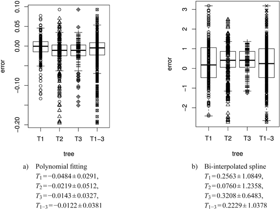
Fig. 13. Error plots [mm2] in box and whisker plots (median, IQR, whiskers at 1.5 IQD or extremal values) of the polynomial and the bi-interpolated spline shape model vs. the original leaf contour of the left leaf side for all individual trees and the average over all trees. The error is calculated as difference between the model and the original leaf contour. The model parameters are individually adapted for each leaf. Below we report the mean ± SD of the respective errors. See list of symbols for further explanations.
Recall that there is no fine-structure biological model underlying our approaches. Rather it can be said that in both approaches, an appropriate model emerges with a set of given parameters. In particular for the low-dimensional proportional model, these parameters have direct geometric meanings.
4.5 Geodesic shape interpolation
The geometric descriptors of shape and size defining a non-symmetrical proportional model as developed in Section 4.3 are identified as 3 two-dimensional landmarks:

Every such 3-landmark configuration x = (x(1), x(2), x(3)) is then viewed as a matrix x / ǁxǁ in the pre shape space S5 ⊆ R2×3 which carries the canonical structure of a non-flat 5-dimensional unit-sphere (Hotz et al. 2010). Within this setup, in order to model growth over one-dimensional time, most parsimonious one-dimensional data descriptors are sought for. Obviously geodesics, i.e. great circles on S5 naturally qualify for this task, as they are generalizations of straight lines to a non-flat structure. A unit-speed geodesic is uniquely determined by initial offset x0 ∈ S5 and initial velocity v0 ∈ S5 orthogonal to x0. Our geodesic model thus is specified as
![]()
where x(t) is the modelled configuration landmark matrix at time t, λ(t) > 0conveys size, γx0,v0 (τ) = x0 cos(τ) + v0 sin(τ) is a great circular geodesic with initial velocity ![]() at γx0,v0 (0) = x0 and τ(t) relates real time with the speed of the geodesic
at γx0,v0 (0) = x0 and τ(t) relates real time with the speed of the geodesic  .
.
As has been shown previously in Hotz et al. (2010), shapes of poplar leaves during growth closely follow geodesics in shape space. As explained below, the proportional model and the geodesic model can be used in conjunction to model rather diversified growth and development.
4.6 Dimensionality of shape and size models
All models introduced here describe leaf form by using a tuple of a one-dimensional size and a multidimensional shape, as is common for biological objects. If we are to model temporal evolution then we may model size as a function of time given by (Eq. 1).
Since in the proportional model, bl / l and br / l are nearly constant in size and lml / l and lmr / l depend rather linearly on size (cf. Section 4.2), for temporal evolution in the proportional model, no new parameter is introduced (of course, using the linear evolution instead of a constant introduces two new parameters (slopes)).
In the polynomial model it turned out that the dependence on length of each of the six coefficients can be well modelled by a sixth order polynomial (cf. Section 4.3.2). In consequence, for temporal evolution, for each leaf side’s shape we have seven parameters.
Although the geodesic model allows for less richness in the modelling of temporal evolution compared to the polynomial model, as with the proportional model, the parameters now have a geometrical meaning: Through every initial point x0 determined by the four parameters of the proportional model (and the current size), there is a four-dimensional space (the tangent space of S5) of possible geodesic directions through x0. Every such direction can be thought of as an individual shape-growing plan of the individual leaf. Indeed, as shown in Hotz et al. (2010), shapes of poplar leaves tend to follow such geodesics rather closely.
The essence of the above considerations is condensed in Table 2. We have included a column for accordingly simplified symmetric models assuming that the right and left leaf side are mirrored.
As explained, all the proposed models have their specific advantages and disadvantages. They differ in number of parameters and the possibility of modelling leaf development over time. Therefore, a final recommendation of the most appropriate model to use in FSPM cannot be made, as it always depends on the specific requirements of the model. The integration of the geodesic as well as the polynomial model would be of great interest for a dynamic FSPM because they allow to model leaf growth over time. In particular the geodesic model is promising as it only requires 9 parameters while the polynomial one needs 85. With respect to computation time the geodesic model is clearly preferable because of fewer parameters. For a static shape model the proportional shape model with only two ratios will be nearly unrivaled.
5 Implementing leaf models as organ modules
5.1 Modelling software and language
For the implementation of our models we used the modelling software GroIMP (Kurth et al. 2006; Kurth 2007; GroIMP Developer Group 2013), with the integrated language XL (Kniemeyer 2004, 2008). This technique can be used for plant modelling in terms of organ modules, where each type of plant organ is implemented as a separate module. The organ modules are reusable program parts that permit a flexible use in different models and rid the modeller of repeatedly having to work out basic aspects such as geometry. These organ modules can be seen as predefined, ready-to-use components which only need to be parameterized appropriately. They lighten the load of low level programming work and thus permit to focus on modelling rather than on coding. Currently two models are available for use in XL in different functional-structural models, a static and a dynamic version.
5.2 Static version
The static leaf model has 10 to 18 input parameters which can be set by the user. First, the tree number has to be chosen to specify which data set is to be used as a base. Then the parameters for the size model (Eq. 1) according to the empirical distribution of Fig. 5 are selected (i). With leaf age as further input (ii) the size of the generated leaf is calculated. To estimate the shape (iii) either the polynomial (Eq. 5) or the proportional model (Sec. 4.2) are chosen. As a last parameter a flag useSawtooth indicates if the additional optical correction is turned on or not. Finally (iv) the contour is obtained according to Hermite or other polynomial interpolation as described above.
The used leaf profile and the trajectory that the leaf vein is following are currently constants but could easily be turned into stochastic functions. The extension of a single leaf (Fig. 14a) depicts as solid black line in the middle the course of the major axis (trajectory) along which the (horizontal) profile is shifted. This will turn the present 2D shape into a curved and bent shape in 3D. In GroIMP e.g. NURBS shapes can be used to visualise the described structure.
5.3 Dynamic version
For the dynamic version time evolution is included. We proceed as for the static version and adapt (iii) to either of:
- pick initial shape and terminal shape parameters from the distribution underlying the proportional model and compute the corresponding geodesic in shape space;
- pick initial shape parameters from the distribution underlying the proportional model and pick a geodesic (future work);
- pick from a distribution underlying the interpolating functions for each parameter of the polynomial model.
Without going into details of the implementation in XL, this leaf module allows to estimate leaf growth over time in an elegant way by simply calling an update() function at each growth step. Internally the age will be increased, other parameters updated and the shape recalculated. For the functional part processes like photosynthesis or transpiration can be run and used to estimate the source and sink behaviour of each leaf independently. For a detailed description of the usage of XL see Kniemeyer (2004, 2008).
5.4 Illustration
To illustrate the possible applications two examples are given: The first is a static structural model (Fig. 14a) of a young poplar tree with a detailed enlargement of a single branch and a single leaf, for which the leaves were produced by the new leaf organ module. To obtain a more realistic 3D impression of the leaf shape a slightly curved bimodal profile was added following the main vein which was modelled as slightly bent. These profiles are based on empirical observation.
A second example (Fig. 14b), based on the model of a young, unbranched poplar (Buck-Sorlin et al. 2008), demonstrates the use of the leaf modules in a more complex functional-structural model, where an accurate leaf area surface is required to calculate the exact amount of light reaching the leaf surface and to estimate the quantity of produced assimilates. The leaf shape was automatically calculated from the age of each leaf.
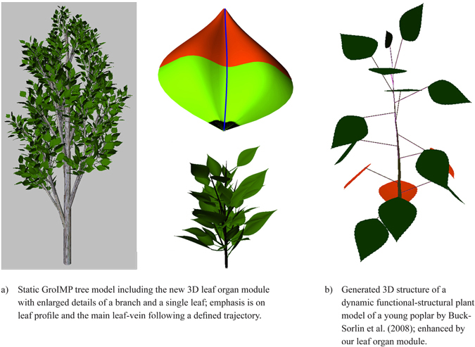
Fig. 14. Two examples integrating the proposed leaf organ module.
6 Conclusions
In this paper a procedure for a non-destructive digitization was developed and demonstrated, using the example of Populus × canadensis leaves. The equipment presented is well suitable for field use, reaching its limits, however, when the investigated objects become too small. Otherwise, there are few restrictions and the methodology can be used for many other species without modification.
A stratified process of image processing was used to extract the contours of the digitized leaves. The image processing tool developed for this purpose, implemented as ImageJ macro, is a semi-automatic tool for contour extraction of leaves of a wide range of broad-leaved plants. Several models were developed based on the data that were collected during one growth cycle. These models are adapted to black poplar and accordingly fitted, but they can be used also for other species with similar leaf shapes, with only a few small changes. Model comparison and validation showed that leaf shape can be well modelled with a small set of parameters. Finally the models were implemented as GroIMP organ modules that can be used in different models as a component.
Providing such modularized systems of predefined leaf organs represents a first step toward a more user-friendly modelling workflow by ridding the modeller from low-level programming work. It thus allows focusing on modelling rather than on coding. As reusable program parts, these organ modules will be included into the library of components of a component-based framework that we are currently working on.
One limitation of the non-destructive method of data acquisition introduced here is that it is only applicable to flat leaves (or those that can be easily flattened), which definitely excludes some species. However, it can be well employed for several other species, including many deciduous trees and crops.
Future work comprises linking the model to environmental parameters like temperature, light quantity and quality, and water. Furthermore, it is envisaged to model leaf damage due to insects or wind.
Acknowledgements
This research was funded by the German Research Foundation (DFG) under project identifier SL 11/12-1. Student assistants Philipp Wree, Julia Rudolph and Julia Knieriem gave support in data acquisition and extraction. S.H. gratefully acknowledges DFG Grant Hu 1575/2. The Department of Tree Physiology and Forest Botany of the University of Göttingen, led by Andrea Polle, provided the sample plants. All assistances are gratefully acknowledged.
References
Biological Modeling and Visualization research group. (2013). The virtual laboratory. [Internet site]. Available at: http://algorithmicbotany.org/virtual_laboratory. [Cited 15 Feb 2014].
Buck-Sorlin G.H., Kniemeyer O., Kurth W. (2008). A model of poplar (Populus sp.) physiology and morphology based on relational growth grammars. In: Deutsch A., Parra R.B. d. l. , Boer R.J. d., Diekmann O., Jagers P., Kisdi E., Kretzschmar M., Lansky P., Metz H. (eds.). Mathematical modeling of biological systems, Volume II. Modeling and Simulation in Science, Engineering and Technology. Birkhäuser, Boston. p. 313–322. http://dx.doi.org/10.1007/978-0-8176-4556-4_28.
Chen C.-C., Chen H., Chen Y.-R. (2009). A new method to measure leaf age: leaf measuring-interval index. American Journal of Botany 96(7): 1313–1318. http://dx.doi.org/10.3732/ajb.0800303.
Chi Y.T., Chien C.F., Lin T.T. (2003). Leaf shape modeling and analysis using geometric descriptors derived from Bezier curves. Transactions of the ASAE 46(1): 175–185.
Chien C.F., Lin T.T. (2005). Non-destructive growth measurement of selected vegetable seedlings using orthogonal images. Transactions of the ASAE 48(5): 1953–1961.
Dennett M.D., Auld B.A., Elston J. (1978). A description of leaf growth in Vicia faba L. Annals of Botany 42(1): 223–232.
De Reffye P., Fourcaud T., Blaise F., Barthelemy D., Houllier F. (1997). A functional model of tree growth and tree architecture. Silva Fennica 31(3): 297–311.
Dornbusch T., Andrieu B. Jan. (2010). Lamina2Shape – an image processing tool for an explicit description of lamina shape tested on winter wheat (Triticum aestivum L.) Computers and Electronics in Agriculture 70(1): 217–224. http://dx.doi.org/10.1016/j.compag.2009.10.009.
Dornbusch T., Watt J., Baccar R., Fournier C., Andrieu B. (2011). A comparative analysis of leaf shape of wheat, barley and maize using an empirical shape model. Annals of Botany 107(5): 865–873. http://dx.doi.org/10.1093/aob/mcq181.
Dryden I.L., Mardia K.V. (1998). Statistical shape analysis. Wiley, Chichester. ISBN 0-4719-5816-1.
Eschenbach C. (2000). The effect of light acclimation of single leaves on whole tree growth and competition – an application of the tree growth model ALMIS. Annals of Forest Science 57(5): 599–609. http://dx.doi.org/10.1051/forest:2000145.
Gallagher J.N. (1979). Field studies of cereal leaf growth. Journal of Experimental Botany 30(4): 625–636. http://dx.doi.org/10.1093/jxb/30.4.625.
Gregory F.G. (1921). Studies in the energy relations of plants. I. The increase in area of leaves and leaf surface of Cucumis sativus. Annals of Botany 35(1): 93–123.
Griffon S., de Coligny F. (2012). AMAPstudio – a software suite for plants architecture modelling. [Internet site]. Available at: http://amapstudio.cirad.fr/doku.php?id=start. [Cited 15 Feb 2014].
GroIMP Developer Group. (2013). Web page of GroIMP. [Internet site]. Available at: http://www.grogra.de. [Cited 15 Feb 2014].
Hackett C., Rawson H. (1974). An exploration of the carbon economy of the tobacco plant. II. Patterns of leaf growth and dry matter partitioning. Australian Journal of Plant Physiology 1: 271–281. http://dx.doi.org/10.1071/PP9740271.
Hotz T., Huckemann S., Gaffrey D., Munk A., Sloboda B. (2010). Shape spaces for pre-aligned star-shaped objects in studying the growth of plants. Journal of the Royal Statistical Society, Series C 59(1): 127–143.
Hu B.G., de Reffye P., Zhao X., Yan H.P., Kang M.Z. (2003). GreenLab: a new methodology towards plant functional-structural model – structural aspect. In: Hu B.G., Jaeger M. (eds.). International Symposium on Plant Growth Modeling, Simulation, Visualization and Applications [PMA03], 2003, Beijing (China PRC), 13–16 October 2003. Tsinghua University Press and Springer, Beijing. p. 21–35.
ImageJ Developer Group. (2013). ImageJ. [Internet site]. Available at: http://rsbweb.nih.gov/ij/index.html. [Cited 15 Feb 2014].
Kniemeyer O. (2004). Rule-based modelling with the XL/GroIMP software. In: Schaub H., Detje F., Brüggemann U. (eds.).The logic of artificial life. Proceedings of 6th GWAL. AKA Akademische Verlagsges Berlin. p. 56–65.
Kniemeyer O. (2008). Design and implementation of a graph grammar based language for functional-structural plant modelling. PhD thesis. BTU Cottbus.
Kniemeyer O., Buck-Sorlin G.H., Kurth W. (2007). GroIMP as a platform for functional-structural modelling of plants. In: Vos J., Marcelis L.F.M., deVisser P.H.B, Struik P.C., Evers J.B. (eds.). Functional-structural plant modelling in crop production. Proceedings of a workshop held in Wageningen (NL), 5.–8. 3. 2006. Springer, Dordrecht. p. 43–52.
Kurth W. (2007). Specification of morphological models with L-systems and relational growth grammars. Image – Journal of Interdisciplinary Image Science 5(1): 50–79.
Kurth W., Buck-Sorlin G.H., Kniemeyer O. (2006). Relationale Wachstumsgrammatiken: Ein Formalismus zur Spezifikation multiskalierter Struktur-Funktions-Modelle von Pflanzen. Modellierung pflanzlicher Systeme aus historischer und aktueller Sicht. Symposium zu Ehren von Prof. Dr. Dr. h.c. E.A. Mitscherlich. Schriftenreihe des Landesamtes für Verbraucherschutz, Landwirtschaft und Flurneuordnung Brandenburg Reihe Landwirtschaft Band 7(1): 36–45.
Lecoustre R., de Reffye P., Jaeger M., Dinouard P. (1992). Controlling the architectural geometry of a plant’s growth – application to the Begonia genus. In: Magnenat Thalmann N., Thalmann D. (eds.). Creating and animating the virtual world. Springer-Verlag New York Inc., New York. p. 199–214.
Maksymowych R. (1973). Analysis of leaf development. Cambridge University Press. ISBN 0-5212-0017-2.
Mosimann J.E. (1970). Size allometry: size and shape variables with characterizations of the lognormal and generalized gamma distributions. Journal of the American Statistical Association 65(330): 930–945.
Neto J.C., Meyer G.E., Jones D.D., Samal A.K. (2006). Plant species identification using elliptic Fourier leaf shape analysis. Computers and Electronics in Agriculture 50(2): 121–134. http://dx.doi.org/10.1016/j.compag.2005.09.004.
Peacock J.M. (1975). Temperature and leaf growth in Lolium perenne. I. The thermal microclimate: its measurement and relation to crop growth. Journal of Applied Ecology 12(1): 99–114.
Perttunen J., Sievänen R., Nikinmaa E., Salminen H., Saarenmaa H., Väkevä J. (1996). LIGNUM: a tree model based on simple structural units. Annals of Botany 77(1): 87–98. http://dx.doi.org/10.1006/anbo.1996.0011.
Prusinkiewicz P., Remphrey W.R., Davidson C.G., Hammel M.S. (1994). Modelling the architecture of expanding Fraxinus pennsylvanica shoots using L-systems. Canadian Journal of Botany 72(5): 701–714. http://dx.doi.org/10.1139/b94-091.
Prusinkiewicz P., Lindenmayer A. (1990). The algorithmic beauty of plants. Springer, New York. ISBN 0-3879-7297-8.
Reich A., Holbrook N.M., Ewel J.J. (2004). Developmental and physiological correlates of leaf size in Hyeronima alchorneoides (Euphorbiaceae). American Journal of Botany 91(4): 582–589. http://dx.doi.org/10.3732/ajb.91.4.582.
Richards F. (1959). A flexible growth function for empirical use. Journal of Experimental Botany 10(2): 290–300. http://dx.doi.org/10.1093/jxb/10.2.290.
Richards F. (1969). The quantitative analysis of growth. In: Steward F.C. (ed.). Plant physiology: a treatise. Analysis of growth. Vol. 5. Series: A. Behaviour of Plants and their Organs. Academic Press, New York. p. 3–76.
Routhier M.-C., Lapointe L. (2002). Impact of tree leaf phenology on growth rates and reproduction in the spring flowering species Trillium erectum (Liliaceae). American Journal of Botany 89(3): 500–505. http://dx.doi.org/10.3732/ajb.89.3.500.
R-Project Developer Group. (2013). The R project for statistical computing. [Internet site]. Available at: http://www.r-project.org. [Cited 15 Feb 2014].
Ruiz-Ramos M., Mínguez M.I. (2006). ALAMEDA, a structural-functional model for Faba Bean crops: morphological parameterization and verification. Annals of Botany 97(3): 377–388. http://dx.doi.org/10.1093/aob/mcj048.
Wiechers D., Kahlen K., Stützel H. (2011). Evaluation of a radiosity based light model for greenhouse cucumber canopies. Agricultural and Forest Meteorology 151(7): 906–915. http://dx.doi.org/10.1016/j.agrformet.2011.02.016.
Yin X., Goudriaan J., Lantinga E.A., Vos J., Spiertz, H .J. (2003). A flexible sigmoid function of determinate growth. Annals of Botany 91(3): 361–371. http://dx.doi.org/10.1093/aob/mcg029.
Total of 40 references

