Annika Kangas  ,
Helena M. Henttonen,
Timo P. Pitkänen,
Sakari Sarkkola,
Juha Heikkinen
,
Helena M. Henttonen,
Timo P. Pitkänen,
Sakari Sarkkola,
Juha Heikkinen
Re-calibrating stem volume models – is there change in the tree trunk form from the 1970s to the 2010s in Finland?
Kangas A., Henttonen H. M., Pitkänen T. P., Sarkkola S., Heikkinen J. (2020). Re-calibrating stem volume models – is there change in the tree trunk form from the 1970s to the 2010s in Finland? Silva Fennica vol. 54 no. 4 article id 10269. https://doi.org/10.14214/sf.10269
Highlights
- TLS data showed that trunk form has changed in Finland from the 1970s
- Significant differences were observed for all tree species
- The trees in TLS data are on average more slender than in the old data.
Abstract
The tree stem volume models of Norway spruce, Scots pine and silver and downy birch currently used in Finland are based on data collected during 1968–1972. These models include four different formulations of a volume model, with three different combinations of independent variables: 1) diameter at height of 1.3 m above ground (dbh), 2) dbh and tree height (h) and 3) dbh, h and upper diameter at height of 6 m (d6). In recent National Forest Inventories of Finland, a difference in the mean volume prediction between the models with and without the upper diameter as predictor has been observed. To analyze the causes of this difference, terrestrial laser scanning (TLS) was used to acquire a large dataset in Finland during 2017–2018. Field-measured predictors and volumes predicted using spline functions fitted to the TLS data were used to re-calibrate the current volume models. The trunk form is different in these two datasets. The form height is larger in the new data for all diameter classes, which indicates that the tree trunks are more slender than they used to be. One probable reason for this change is the increase in stand densities, which is at least partly due to changed forest management. In models with both dbh and h as predictors, the volume is smaller a given h class in the data new data than in the old data, and vice versa for the diameter classes. The differences between the old and new models were largest with pine and smallest with birch.
Keywords
TLS;
OLS;
regression;
terrestrial laser scanning
-
Kangas,
Natural Resources Institute Finland (Luke), Yliopistokatu 6 B, FI-80100 Joensuu, Finland
 https://orcid.org/0000-0002-8637-5668
E-mail
annika.kangas@luke.fi
https://orcid.org/0000-0002-8637-5668
E-mail
annika.kangas@luke.fi
- Henttonen, Natural Resources Institute Finland (Luke), Latokartanonkaari 9, FI-00790 Helsinki, Finland E-mail helena.henttonen@luke.fi
-
Pitkänen,
Natural Resources Institute Finland (Luke), Latokartanonkaari 9, FI-00790 Helsinki, Finland
https://orcid.org/0000-0001-5389-8713
E-mail
timo.p.pitkanen@luke.fi
- Sarkkola, Natural Resources Institute Finland (Luke), Latokartanonkaari 9, FI-00790 Helsinki, Finland E-mail sakari.sarkkola@luke.fi
-
Heikkinen,
Natural Resources Institute Finland (Luke), Latokartanonkaari 9, FI-00790 Helsinki, Finland
https://orcid.org/0000-0003-3527-774X
E-mail
juha.heikkinen@luke.fi
Received 12 November 2019 Accepted 16 September 2020 Published 18 September 2020
Views 52205
Available at https://doi.org/10.14214/sf.10269 | Download PDF

Supplementary Files
Corrections
1 Introduction
In Finland, the stem volume models developed by Laasasenaho (1982) have been used in National Forest Inventory (NFI) since the models were estimated, and in all forest inventory and planning applications since they were published in 1982. The data were used to develop several different volume models with varying combinations of diameter at breast height (dbh, diameter at height of 1.3 m above ground), height (h), and diameter at height of 6 m (d6) as predictors. The data were also utilized to model taper curves with a continuous polynomial function of height (Lahtinen and Laasasenaho 1979; Laasasenaho 1982). Later on, the same dataset was also used to model taper curves using a mixed models approach (Lappi 1986; Korhonen 1991). In the latest application, the taper curve was predicted with a non-parametric approach involving random effects (Lappi 2006).
The data (in the following named old data) for the current stem volume models were collected in 1968–1972 from the plots of the 5th National Forest Inventory in Finland (NFI). In more recent NFIs, it has become obvious that the mean difference in the volume estimates between the models with (dbh, h) and (dbh, h, d6) as predictors is not zero, indicating that the form of the trees trunks has changed from the 5th NFI. The difference is varying from region to region, and it seems to be increasing in time (Fig. 1). Therefore, it was deemed important to analyze if the change in the tree trunk form is real; and re-calibrate the old volume models if needed.
The old data was collected mainly from standing trees, by climbing the trees (Laasasenaho 1982). Nowadays, such method is not feasible anymore. Instead, in recent years, stem data collected by Terrestrial Laser Scanning (TLS) has been utilized in many occasions, in construction of volume and biomass models (Calders et al. 2015; Saarinen et al. 2017, 2019; Liang et al. 2018). Inspired by these earlier studies, a decision to collect a TLS dataset for volume modelling was made, and representative data covering most parts of Finland were collected during 2017–2018. First, a method to estimate diameters at different heights from the scanned trees was developed (Pitkänen et al. 2019), and second, the method was used to predict the taper curves of the trees. The method was validated using 74 felled and field-measured trees and based on the achieved results it was deemed suitable for estimating new volume models (Pitkänen et al. 2020). The main validation criteria was the observed systematic error of volume estimates, which would cause a mis-specified volume model, while random errors will only increase the model residual errors (Kangas 1998).
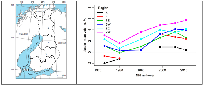
Fig. 1. The difference between the predictions of the two volume models from the 1970s to the 2010s (right) by the National Forest Inventory of Finland (NFI) sampling region (left). Sampling regions 2 and 3 are divided into western (W) and eastern (E) parts.
The aim of this study is to analyze if the TLS data provide evidence of tree trunk shape changing in time. To this end, we analyzed the form heights of the trees in the old and new data sets. We also re-calibrated the old stem volume models for the three main tree species in Finland. We used the methods developed earlier, for estimating the taper curves from the TLS data (Pitkänen et al. 2019, 2020). The old volume models with dbh or dbh and h as predictors were chosen to be re-calibrated, as the model with d6 included described the tree form adequately without re-calibrating in the validation (Pitkänen et al. 2020). As our goal was to estimate the change in the tree trunk form between the datasets, we used a combined data together with a parametrization that enabled the assessment of statistical significance of changes.
The published model with dbh and h as predictors is not suitable for small trees, i.e. tree less than 3 meters high for conifers and 4 meters high for birch (Laasasenaho 1982). This is largely due to using ln(h–1.3) as one predictor: the value of this predictor approaches infinity as height approaches 1.3 meters. Therefore, we estimated also the coefficients for a model form previously used to model the volume for small trees in NFI (Tomppo et al. 2011), which behaves more logically with small heights.
2 Material
Our study material consists of two datasets: 1) The old data including 2326 Scots pine (Pinus sylvestris L.), 1864 Norway spruce (Picea abies L. Karst. ) and 863 silver (Betula pendula Roth) and downy (Betula pubescens Ehrh.) birches, collected from the 5th National Forest Inventory (NFI) field plots during 1968–1972, throughout the whole Finland (Laasasenaho 1982), and 2) new data, collected from the 12th National Forest Inventory field plots using TLS during 2017–2018.
For TLS data collection, a sample of 200 clusters of NFI field plots was selected with the goal to measure a balanced sample of approximately 4000 trees in different conditions. Åland and the Northern Lapland (regions 1 and 6 in Fig. 1 covering 4.2% of the forestry area) were excluded due to their special conditions. It was assumed that during one day, the field group could measure and scan 1–3 plots, and therefore, three plots from each cluster were selected to the sample.
The NFI measurements were utilized as auxiliary information in order to secure a well-spread sample of TLS plots from the target population. First, the temporary clusters measured in NFI during 2016 were divided to sampling strata based on soil type (peatland/mineral), basal area weighted mean diameter and proportion of birch from the basal area in order to ensure similar representation of less common peatlands, large trees, and birch as observed in NFI. Within each NFI sampling region (Fig. 1), the clusters were first divided to those that include peatland plots and those that do not, then within the resulting strata to those with mean diameter above/below the upper quartile, and finally to those with above/below median birch proportion (Supplementary file S1). The sample was divided to sampling regions based on the proportion of total volume, and to strata proportionally to their area. Local pivotal method (Grafström et al. 2012) was applied to obtain a geographically balanced sample of fixed size from the irregular population of 2016 NFI clusters within each stratum (Suppl. file S2). The three plots from each sampled cluster were selected as those with minimum, median, and maximum basal area. Only those plots from which pine, spruce, or birch trees were measured in NFI were considered as candidates. When there were 1–3 such plots in a sampled cluster, they were all selected.
The end result was a sample of 200 clusters of three plots throughout the Finland (Fig. 2). In 2017 altogether 102 plots were measured, and in 2018 151 plots, i.e. totally 253 plots (out of the goal of 552 plots). Each plot was scanned using 4–5 stations, which were placed with intention to ensure the visibility of sample trees from several directions. The sample trees were selected using a relascope plot (Bitterlich 1948) with basal area factor q = 2. All living trees were included, but in practise only trees higher than 4 meters were detected from the scanned data. Before scanning, the selected trees were marked with a duct tape placed 10 cm above the breast height, allowing for determining the correct ground level and breast height from the scanning data. From each tree, stump height, stump height diameter, dbh and h were measured in the field and used to assist in the TLS-based stem volume predictions. This was carried out to mitigate errors noted in earlier TLS studies, for instance underestimation of height (Saarinen et al. 2017; Pitkänen et al. 2019, 2020). The field-measured values of dbh and h were also used as predictors in the estimated models.
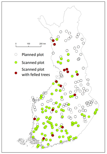
Fig. 2. The plots selected for TLS data collection (all dots), scanned plots (green dots), felled trees (red dots).
The data consisted of 2168 scanned trees, out of which 971 were Scots pine, 687 Norway spruce, 405 downy or silver birch and 105 other tree species. After processing the point cloud data (Pitkänen et al. 2019, 2020), some of the scanned trees were discarded due to weak quality of TLS data (caused by e.g. occlusions). In the end, 246 plots and 1968 trees were accepted for modelling (Table 1). From these, only pines, spruces and birches on forest land were included in the modelling in order to mimic the old study (see below).
| Table 1. The minimum, maximum and mean of diameter at breast height (dbh), height (h) and volume (v) in the old and new volume modelling data by tree species. | |||||||
| old data | new data | ||||||
| min | max | mean | min | max | mean | ||
| pine | dbh (cm) | 0.90 | 50.60 | 20.23 | 3.90 | 49.70 | 20.90 |
| h (m) | 1.50 | 28.30 | 13.67 | 5.40 | 29.60 | 16.59 | |
| v (dm3) | 0.40 | 1921 | 312 | 5.10 | 1947.7 | 340.20 | |
| spruce | dbh (cm) | 1.5 | 61.9 | 18.04 | 5.55 | 57.00 | 22.25 |
| h (m) | 1.8 | 32.7 | 13.82 | 4.50 | 32.70 | 18.19 | |
| v (dm3) | 0.7 | 3796 | 264 | 7.40 | 2856.4 | 448.20 | |
| birch | dbh (cm) | 1.2 | 49.7 | 16.65 | 4.00 | 42.45 | 16.18 |
| h (m) | 2.4 | 29.5 | 15.33 | 4.50 | 29.80 | 16.20 | |
| v (dm3) | 0.4 | 2026 | 229 | 4.30 | 1427.70 | 213.36 | |
In the old study (Laasasenaho 1982), only trees on forest land were used for modelling resulting 2050 pines, 1841 spruces and 834 birches. The non-forest land trees were excluded due to non-representative data for this group (Laasasenaho 1982 p. 41). The trees to be measured were selected with a relascope (q = 2). However, the number of trees measured per plot was restricted to 5 trees (using an unspecified rule Laasasenaho 1982 p. 9). Trees with dbh ≤ 10 mm i.e. three pines, were rejected from the modelling data, and the same trees were discarded also in this study.
The volumes of the trees were predicted using cubic spline to interpolate the taper curve, and the result was integrated as (Lahtinen and Laasasenaho 1979):
![]()
where s denotes the diameter as the function of height, and h is the height of the tree and 0is the stump height level. The data properties are described in Table 1.
In formulating the taper curves from the TLS data, taper curve models estimated with the method presented by Lappi (1986, 2006) were used as a prior information, to prevent substantial under- or overestimates of the TLS-based stem diameters (Pitkänen et al. 2020). The reference taper curves were estimated from two independent data sets (Korhonen and Maltamo 1990; Varjo et al. 2006).
The final taper curves were predicted using cubic splines in the same way as in the original study (Laasasenaho 1982; Pitkänen et al. 2020). TLS-based stem volumes above the stump height were predicted using the cubic spline and Huber formula (Husch et al. 1972) with 1 cm slices. This method approximates numerical integration.
3 Methods
For the comparisons of the old and new tree datasets, the calculations were done in two steps. Firstly, the form height:

by tree species and dataset was estimated. It describes the ratio of volume (v) and basal area (g) of the tree. The form heights were compared by diameter classes to analyze possible changes. The diameter classes were formed from the percentiles (0, 10%, 20%, 30%, 40%, 50%, 60%, 70%, 80%, 90%, 100%) of diameter in the old data set.
Secondly, the published models by Laasasenaho (1982) were re-calibrated. To preserve comparability of the new models with the published ones, exactly the same model forms and methods were used. This means that all models were fitted by ordinary least squares. Log transformation of volume was in all cases used to account for the obvious heteroscedasticity of the data.
The original models had the general form:
![]()
where the potential predictors xki include dbh and h of tree i and their monotonic transformations. The models were fitted to the combined data set containing the trees from both old and new data.
To describe difference between the coefficients in the old data and the new data, the models were re-parametrized into:
![]()
where λi = 1 if tree i is from the new data, and λi = 0, if it is from the old data. Thus β’s are the coefficient values describing the old data and δ’s indicate the difference between the coefficient values of new and old data. To investigate whether including the difference between the two datasets significantly improved the fit, an F-test to compare the original (3) and full (4) model was made. The significance of improvement due to any single variable was not considered at all, in order to prevent some of the possible effect of the new data to be confused with the effect of the original data. The reported estimated values of the intercept coefficient β0 include bias correction term ![]() (Flewelling and Pienaar 1981), where
(Flewelling and Pienaar 1981), where ![]() is the estimated residual variance, so that the back-transformed volume predictions are approximately unbiased.
is the estimated residual variance, so that the back-transformed volume predictions are approximately unbiased.
As OLS models with correlated observations may inflate the F-test values, the same models were also estimated using a mixed model with a plot effect to describe the within-plot correlations. To investigate whether including the difference between the two datasets significantly improved the fit, a likelihood ratio test was used in the same way as F-test in the OLS setting.
Volume models considered in this study were:
![]()
![]()
![]()
![]()
Models (5)–(7) correspond to equations (61.1)–(61.3) in Laasasenaho (1982), and model (8) was presented as equation 3.20 for small trees in (Tomppo et al. 2011). Note that equation 3.20 is not correct in Tomppo et al. (2011, p. 77) (ln(dbh) assumed instead of dbh), but the coefficients in table 3.5 refer to model (8) presented here.
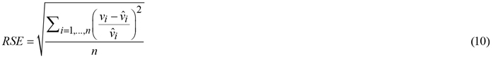
Also the relative standard errors were estimated in the same way as in the original study using the formula (Laasasenaho 1982)
![]()
where ![]() is the estimated residual variance. In this study the relative standard errors were also estimated using the formula proposed by Lappi (1986):
is the estimated residual variance. In this study the relative standard errors were also estimated using the formula proposed by Lappi (1986):
The residuals of the models with and without the effect of the new data by diameter classes were analyzed in the new dataset. This reveals how well the old model performs in a new era and how much of the possible errors the new model can reduce.
4 Results
The form height of trees was larger in the new data than in the old data in all diameter classes for all tree species (Fig. 3). For birch the difference was smallest, for pine largest. It indicates that for a given diameter, the tree volumes in the new data are larger in all diameter classes.
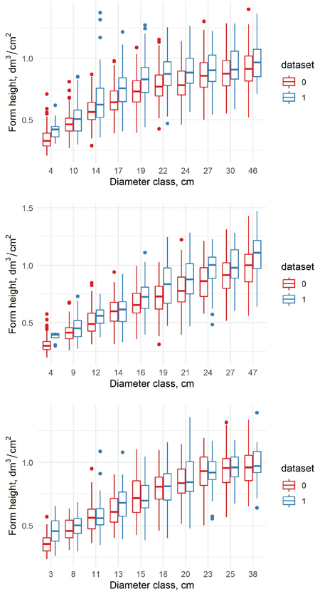
Fig. 3. The form height in old (0) and new (1) dataset for pine (upper) spruce (middle) and birch (lower) in the percentile diameter classes.
The estimated coefficients, their standard errors and t-values for the equation (5), and the originally estimated coefficients of the old model using OLS are presented in Table 2. While the F-test shows (Table 3) that the added variables describing the new data significantly improve the fit as a whole, single coefficients not necessarily do. Unfortunately, the standard errors and coefficients of determination were not presented in (Laasasenaho 1982). For the old model, these statistics were thus estimated by fitting the old models again to the old data (Table 3). The relative standard errors of the new models are very close to the old ones with all species. The differences in the predictions are fairly small in all species, which is largely due to the fact that only one independent variable is included. For pine and spruce the volumes predicted with the new model were larger for a given diameter than in the old model. For birch, the volumes were very close to each other.
| Table 2. The estimates of coefficients of the volume model 5 (61.1. in Laasasenaho 1982), their standard error and t-values for all species | |||||
| full data model | old model | ||||
| coefficient | standard error | t-value | coefficient | ||
| pine | β0 | –2.293114 | 0.0228019 | –101.3275 | –2.29450 |
| β1 | 2.570253 | 0.007707629 | 333.4687 | 2.57025 | |
| δ0 | 0.2105365 | 0.05147734 | 4.089886 | ||
| δ1 | –0.03352298 | 0.01723158 | –1.945438 | ||
| spruce | β0 | –2.411956 | 0.02326293 | –104.5267 | –2.41218 |
| β1 | 2.624621 | 0.008255297 | 317.9317 | 2.62463 | |
| δ0 | 0.06596944 | 0.06211427 | 1.062066 | ||
| δ1 | 0.009008474 | 0.0206251 | 0.4367724 | ||
| birch | β0 | –2.102088 | 0.03392367 | –62.55514 | –2.09787 |
| β1 | 2.55162 | 0.01231355 | 207.2205 | 2.55058 | |
| δ0 | 0.1252633 | 0.06947937 | 1.802885 | ||
| δ1 | –0.03105756 | 0.02547401 | –1.219186 | ||
| Table 3. The residual standard error (RSE) and the coefficient of determination (Multiple R2) for old and new volume models (5) by species. The F-test describes the significance of the full model compared to the old model. | ||||||||
| Tree species | Full data | Old data | ||||||
| RSE original | RSE | Multiple R2 | F-test | p-value | RSE original | RSE | Multiple R2 | |
| Pine | 19.51 | 19.45 | 0.9792 | 115.36 | 0 | 18.01 | 17.81 | 0.9833 |
| Spruce | 20.41 | 20.93 | 0.9811 | 48.768 | 0 | 19.91 | 20.77 | 0.9823 |
| Birch | 20.30 | 19.88 | 0.9792 | 6.1824 | 0.002 | 20.08 | 19.66 | 0.9812 |
The relative residuals of the old and new model were analyzed only in the new data, to show potential problems of the old models in the new era. When the relative residuals are analyzed by diameter classes, the old model underestimates the volumes in the largest diameter classes but overestimates in the middle diameter classes for pine (Fig. 4). For spruce, the pattern is quite similar. For birch, the old model overestimates the volumes in the smallest diameter classes and underestimates in the largest diameter classes, but the differences between the diameter classes are relatively small. Our new model is able to correct the general level, but it cannot correct the differences between the diameter classes due to the fixed model shape.
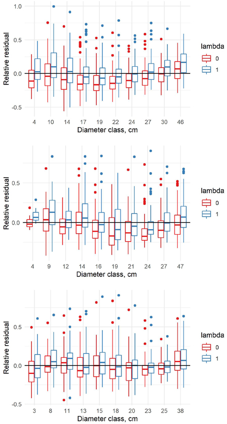
Fig. 4. Relative residuals of model 5 in the dbh classes of the new data with λ = 0 and λ = 1 for pine (upper row), spruce (middle row) and birch (lower row).
The estimated coefficients, their standard errors and t-values for the equation (6), and the originally estimated coefficients of the old model are presented in Table 4, and the F-tests, standard errors and coefficients of determination in Table 5. Similarly as for equation (5), while according to the F-test the added variables significantly improved the fit as a whole, the same was not true for all added variables. Also with this model, volumes with a given diameter are larger than in the old data for pine, but vice versa for large spruces. For birch this model form shows a large difference for the largest trees. It is notable that according to the study by Zianis et al. (2005), the published formula for pine (Laasasenaho 1982) differed clearly from all published volume models for pine in the whole Europe. It can also be noted from Fig. 5 that this equation (6) gives clearly smaller volumes for largest trees than equation (5).
| Table 4. The estimates of coefficients of the volume model 6 (61.2. in Laasasenaho 1982), their standard error and t-values for all species | |||||
| full data model | old model | ||||
| coefficient | standard error | t-value | coefficient | ||
| pine | β0 | –5.392811 | 0.06715021 | –80.54965 | –5.39417 |
| β1 | 3.480598 | 0.03040095 | 114.4898 | 3.48060 | |
| β2 | –0.03198842 | 0.001596443 | –20.03731 | –0.039884 | |
| δ0 | –0.002811802 | 0.1647923 | –0.0170627 | ||
| δ1 | 0.06637664 | 0.07175107 | 0.9250962 | ||
| δ2 | –0.005370931 | 0.003522453 | –1.52477 | ||
| spruce | β0 | –5.398914 | 0.06499235 | –83.34407 | –5.39934 |
| β1 | 3.46464 | 0.03031531 | 114.2868 | 3.46468 | |
| β2 | –0.02731815 | 0.001716997 | –15.91042 | –0.0273199 | |
| δ0 | –0.4109449 | 0.2124345 | –1.934454 | ||
| δ1 | 0.2087533 | 0.08939057 | 2.335294 | ||
| δ2 | –0.00843131 | 0.004000025 | –2.107814 | ||
| birch | β0 | –5.327978 | 0.08839265 | –60.48643 | –5.41948 |
| β1 | 3.546208 | 0.04242831 | 83.58118 | 3.57630 | |
| β2 | –0.03882196 | 0.002573179 | –15.08716 | –0.0395855 | |
| δ0 | –5.327978 | 0.08839265 | –60.48643 | ||
| δ1 | 3.546208 | 0.04242831 | 83.58118 | ||
| δ2 | –0.03882196 | 0.002573179 | –15.08716 | ||
| Table 5. The residual standard error (RSE) and the coefficient of determination (Multiple R2) for old and new volume models (6) by species. The F-test describes the significance of the full model compared to the old model. | ||||||||
| Tree species | Full data | Old data | ||||||
| RSE original | RSE | Multiple R2 | F-test | p-value | RSE original | RSE | Multiple R2 | |
| Pine | 18.09 | 17.77 | 0.9807 | 69.078 | 0 | 17.30 | 17.04 | 0.9846 |
| Spruce | 19.04 | 18.45 | 0.9829 | 38.97 | 0 | 18.86 | 18.42 | 0.9841 |
| Birch | 19.27 | 18.54 | 0.9811 | 8.3378 | 0 | 18.89 | 18.08 | 0.9834 |
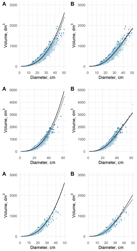
Fig. 5. The predicted tree volumes as a function of dbh in old data (light blue dots) and new data (blue dots) for pine (upper), spruce (middle) and birch (lower) using model 5 (A) and model 6 (B). Black curve is based on new data and grey on the old data.
When analyzed in the new data by diameter classes, the relative residuals of the old model are overestimates for all diameter classes for pine and spruce. The overestimates are larger in the middle diameter classes (Fig. 6). For birch, the pattern is less clear. Also here, the new model can correct the general level, but not the differences between the diameter classes due to the fixed model shape.
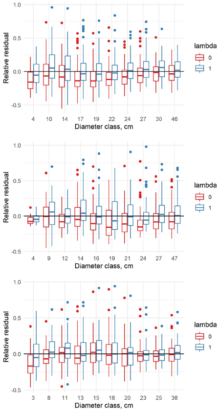
Fig. 6. Relative residuals of model 6 in the dbh classes of the new data with λ = 0 and λ = 1 for pine (upper row), spruce (middle row) and birch (lower row).
The estimated coefficients, their standard errors and t-values for the equation (7), and the originally estimated coefficients of the old model are presented in Table 6, and the F-tests, standard errors and coefficients of determination in Table 7. The predicted volumes in the old data and new data differ in a sense that when conditioned on diameter, the volumes in the new data are larger except for largest spruces. The differences are small for small diameter classes, but more clear in largest diameter classes. When conditioned on height, the volumes in the new data are smaller for all tree species (Fig. 7). The differences are much more clear with respect to the height classes. This confirms that the form of the trunks is different between these two datasets, and especially the role of height is different.
| Table 6. The estimates of coefficients of the volume model 7 (61.3. in Laasasenaho 1982), their standard error and t-values for all species. | |||||
| full data model | old model | ||||
| coefficient | standard error | t-value | coefficient | ||
| pine | β0 | –3.383341 | 0.04207626 | –80.45867 | –3.32176 |
| β1 | 2.015408 | 0.01445914 | 139.3864 | 2.01395 | |
| β2 | 2.144271 | 0.05597404 | 38.30831 | 2.07025 | |
| β3 | –1.121108 | 0.04888704 | –22.93263 | –1.07209 | |
| β4 | –0.004035521 | 0.0006782147 | –5.950211 | –0.003273 | |
| δ0 | 0.5831496 | 0.1432678 | 4.070347 | ||
| δ1 | –0.1778505 | 0.03040952 | –5.848513 | ||
| δ2 | –1.1444 | 0.2984041 | –3.835067 | ||
| δ3 | 1.141898 | 0.2689587 | 4.245627 | ||
| δ4 | 0.002406294 | 0.001429594 | 1.683201 | ||
| spruce | β0 | –3.782985 | 0.04199002 | –90.15069 | –3.77543 |
| β1 | 1.912913 | 0.01687974 | 113.326 | 1.91505 | |
| β2 | 2.833072 | 0.04900075 | 57.81691 | 2.82541 | |
| β3 | –1.538206 | 0.04188057 | –36.7284 | –1.53547 | |
| β4 | –0.008581622 | 0.0008074753 | –10.62772 | –0.0085726 | |
| δ0 | 0.03531895 | 0.1722487 | 0.2050462 | ||
| δ1 | –0.0461456 | 0.04193549 | –1.100395 | ||
| δ2 | 0.1403905 | 0.3540179 | 0.3965632 | ||
| δ3 | –0.1161943 | 0.3197521 | –0.3633886 | ||
| δ4 | 0.0003250218 | 0.001790375 | 0.1815384 | ||
| birch | β0 | –4.553696 | 0.08843668 | –51.52675 | –4.49213 |
| β1 | 2.122157 | 0.02553022 | 83.12333 | 2.10253 | |
| β2 | 4.096565 | 0.1526368 | 26.83864 | 3.98519 | |
| β3 | –2.767257 | 0.1362035 | –20.31707 | –2.65900 | |
| β4 | –0.01485222 | 0.001453626 | –10.21736 | –0.0140970 | |
| δ0 | 0.4878564 | 0.2303936 | 2.117491 | ||
| δ1 | –0.2301959 | 0.04762161 | –4.833855 | ||
| δ2 | –0.5090479 | 0.5184651 | –0.9818365 | ||
| δ3 | 0.4926584 | 0.4648618 | 1.059795 | ||
| δ4 | 0.01209118 | 0.002811613 | 4.300443 | ||
| Table 7. The residual standard error (RSE) and the coefficient of determination (Multiple R2) for old and new volume models (7) by species. The F-test describes the significance of the full model compared to the old model. | ||||||||
| Tree species | Full data | Old data | ||||||
| RSE original | RSE | Multiple R2 | F-test | p-value | RSE original | RSE | Multiple R2 | |
| Pine | 6.42 | 6.42 | 0.9975 | 32.933 | 0 | 6.82 | 6.81 | 0.9976 |
| Spruce | 7.00 | 6.97 | 0.9977 | 7.7947 | 0 | 7.46 | 7.42 | 0.9975 |
| Birch | 7.96 | 7.88 | 0.9967 | 10.531 | 0 | 8.13 | 7.98 | 0.9969 |
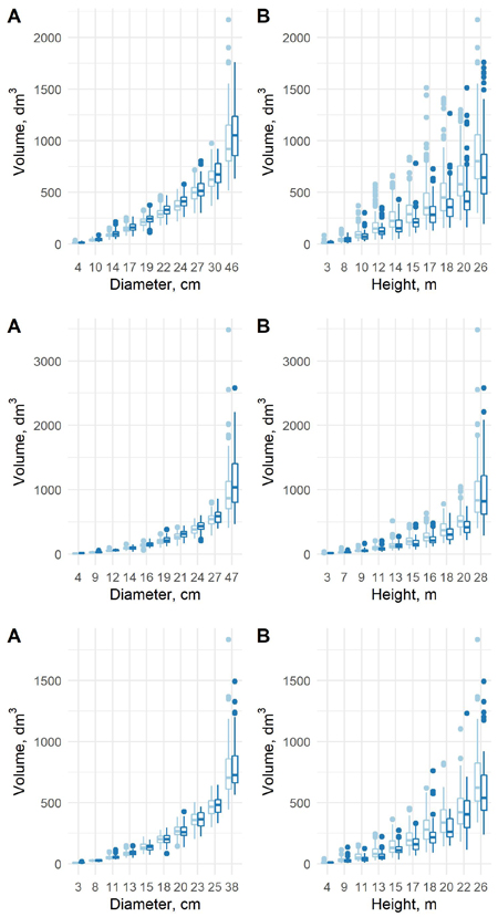
Fig. 7. The predicted tree volumes using model 7 in the old data (light blue) and new data (blue) as a function of dbh class (A) and h class (B) for pine (upper row), spruce (middle row) and birch (lower row).
The relative residuals of the model were estimated in the new data set. For pine and spruce the old model underestimates the volumes in the largest diameter classes of the new data (Fig. 8). For birch the old model overestimates the volumes in the smallest diameter class and underestimates in all other classes. The new coefficients can to some extent adjust the model to the new data.
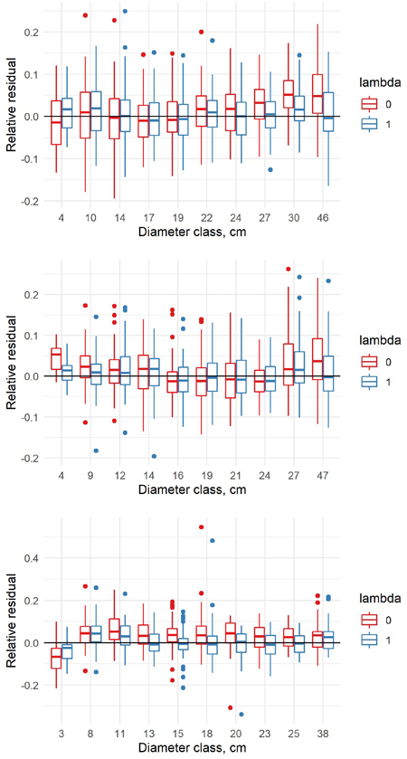
Fig. 8. Relative residuals of model 7 in the dbh classes of the new data with λ = 0 and λ = 1 for pine (upper row), spruce (middle row) and birch (lower row).
The estimated coefficients, their standard errors and t-values for the equation (8) are presented in Table 8, and the F-tests, standard errors and coefficients of determination in Table 9. With the new model form, the predicted volumes in the old data (λ = 0) and new data (λ = 1) differ in a similar way as in the previous model. When conditioned on diameter, the volumes in the new data are larger, and when conditioned on height, the volumes in the new data are smaller (Fig. 9). For pine and spruce, the old model underestimates the volumes in the largest and smallest diameter classes of the new data and overestimates them in the middle classes (Fig. 10). For birch the old model overestimates the volumes in the smallest diameter class and underestimates them in other classes. The new model appears adequate for all tree species, even though it is not as accurate as the previous model.
| Table 8. The coefficients, their standard errors and t-values of the new volume model (8) for all species. | ||||
| full data model | ||||
| coefficient | standard error | t-value | ||
| pine | β0 | –4.447527 | 0.02631802 | –169.0749 |
| β1 | 2.362339 | 0.01531425 | 154.2575 | |
| β2 | –0.01054031 | 0.0006214953 | –16.9596 | |
| β3 | 0.8566598 | 0.007997866 | 107.111 | |
| δ0 | –0.05472306 | 0.06228864 | –0.87854 | |
| δ1 | –0.1009865 | 0.03211809 | –3.144226 | |
| δ2 | –0.002319712 | 0.001344036 | –1.72593 | |
| δ3 | 0.1566015 | 0.01423715 | 10.9995 | |
| spruce | β0 | –4.162928 | 0.03039662 | –137.0555 |
| β1 | 2.083863 | 0.01977891 | 105.3578 | |
| β2 | –0.00527749 | 0.0007558304 | –6.982374 | |
| β3 | 1.040583 | 0.0114666 | 90.74904 | |
| δ0 | –0.207592 | 0.09298762 | –2.232469 | |
| δ1 | 0.007377705 | 0.04845477 | 0.1522596 | |
| δ2 | –0.005278365 | 0.001738939 | –3.035395 | |
| δ3 | 0.1034346 | 0.02262765 | 4.57116 | |
| birch | β0 | –5.12979 | 0.04217144 | –121.7211 |
| β1 | 2.509713 | 0.02722397 | 92.18763 | |
| β2 | –0.02113233 | 0.001285776 | –16.43546 | |
| β3 | 0.9830402 | 0.01676183 | 58.64755 | |
| δ0 | 0.2926902 | 0.09660794 | 3.02967 | |
| δ1 | –0.2129817 | 0.05494384 | –3.876353 | |
| δ2 | 0.009456602 | 0.002737932 | 3.453922 | |
| δ3 | 0.06331147 | 0.02997322 | 2.112268 | |
| Table 9. The residual standard error (RSE) and the coefficient of determination (Multiple R2) for old and new volume models (8) by species. The F-test describes the significance of the full model compared to the old model. | |||||
| Tree species | Full data | ||||
| RSE original | RSE | Multiple R2 | F-test | p-value | |
| Pine | 6.62 | 6.67 | 0.9974 | 41.096 | 0 |
| Spruce | 7.88 | 8.13 | 0.9970 | 12.158 | 0 |
| Birch | 8.22 | 8.19 | 0.9965 | 9.1126 | 0 |
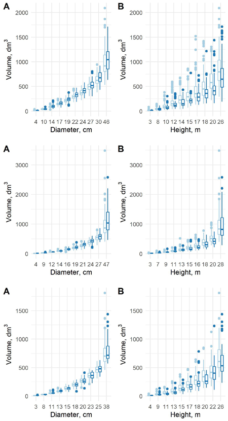
Fig. 9. The predicted tree volumes with the new model 8 in the old data (light blue) and new data (blue) as a function of dbh class (A) and h class (B) for pine (upper row), spruce (middle row) and birch (lower row).
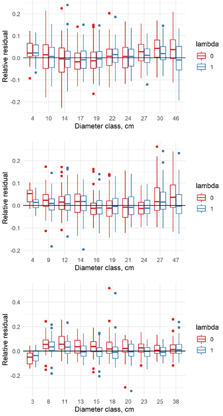
Fig. 10. Relative residuals of model 8 in the dbh classes of the new data with λ = 0 and λ = 1 for pine (upper row), spruce (middle row) and birch (lower row).
When the models (5–8) were estimated using a mixed model approach, the coefficients in both the old and new data differed markedly from the published ones (Suppl. file S3). Therefore, we used the mixed models only to check the validity of the F-tests. Based on the mixed models and likelihood ratio test, the difference is significant for pine and spruce but not significant for birch except for one model (7). This confirms the evidence of a changed tree trunk form for pine and spruce. The small change of tree trunk form for birch was also evident from the OLS analysis.
5 Discussion
In this study, we used the volumes predicted using TLS data to re-calibrate the coefficients for the published volume models. The aim is that all forest practitioners having been using the old models can now choose between the old and the new coefficients, while the model forms remain similar as before. It also makes the changes in the tree form easier to interpret.
Our goal was to analyze, if there is evidence regarding the change in the stem trunk form since the beginning of the 1970s. The results in this sense are distinct; there is a significant change in the trunk form in the two datasets, as the additional coefficients significantly improved the fit according to the F-test in all models. When the validity of the F-tests related to observations correlated within the plots was checked, the conclusions of changed tree trunk form were confirmed. With birch, where the changes were also visually very small, the change is not significant when the correlations are accounted. The tree trunk form of birch having not changed significantly in time can also be interpreted as evidence that using TLS data as such does not cause the differences.
In the more complicated model equations (7) and (8), the differences in different coefficients could be to opposite directions, so that interpreting the changes is not trivial. However, the changes can be clearly detected from the mean predictions within the diameter and height classes. It is notable that the differences are clearer when the predictions are compared across the height classes. It indicates that especially the role of height in the volume models is different compared to the old data.
In many cases, the differences varied across the diameter classes. For pine and spruce, for instance, the old model equation (7) underestimated the volumes in the largest diameter class, but overestimated them in the middle classes. Obviously, the largest trees were young trees when the old data was collected, so that it is possible that the changes in the trunk form are most evident in the smaller diameter classes. Apparently, the form of trees changes gradually, due to the changing growing conditions and changing forest management. For analyzing the changes in more detail in future, we will introduce a third dataset, measured in the 1990s, and test the models estimated here in the independent data. This will give new insights on the timeline and causes of the changes. The gradual change also means that the volume models need to be updated again when the largest diameter classes have been felled and the current middle diameter classes are the largest tree classes. It is also possible that some model equation forms can handle the change better than others, i.e. some predictors may be more resistant to the change than others.
In this study, we only analyzed the tree volumes as total. Therefore, it is not possible to detect from these results, in which part of the stem the observed changes have occurred. This can be analyzed, when the taper curves of (Laasasenaho 1982) are also recalibrated and the results analyzed. It is also possible, that depending on the forest management, part of the trees are more slender than before and part are less slender. This is also a question that needs to be answered in the future.
We chose to make the model using both the old and new datasets also in order to obtain stable estimates of the coefficients, as the new data set is smaller than the old one, and there is an area lacking new measurements particularly in North-Eastern Finland (due to lacking funding). However, the new models (with λ = 1) seem to produce results with an acceptable mean error in all diameter classes of the new data.
There are indications of regional differences in the temporal change of the stem form (Fig. 1). Therefore, in the future it is important to make completely new kind of volume models, where this regional variation can be accounted for. It would be possible to model the volumes in the future using non-linear models with locally adjustable parameters or even model the parameters as function of the coordinates (Mehtätalo et al. 2015).
All predictors used in the models were field-measured, meaning the accuracy between the old data and the new data can be assumed similar in this sense. Therefore, the errors-in-variables are not causing bias that needs to be accounted: if the models are used with application data that are measured with similar equipment, the bias resulting from the measurement errors can be ignored (Kangas 1998). On the other hand, we assumed that the volumes predicted using TLS data and those predicted using measurements obtained by climbing the trees were as precise. Although random estimates can cause bias in the volume estimates used for modelling, we had to assume this effect negligible due to lacking information of the measurement accuracy at different heights of the stems. This assumption is supported by the fact that in a validation study, including the upper diameter in the volume model was able to prevent systematic errors in the results (Pitkänen et al. 2020). If the systematic errors were due to problems in TLS data, including the upper diameter would not have had such effect. In the future, there is possibly a need to address the varying measurement errors in the dataset in the modelling. One option would be to estimate the models as hierarchical Bayesian models, where the distribution of measurement errors is accounted for. Introducing a new dataset with different measurement technique from the 1990s might also give further insight into this potential problem.
6 Conclusion
The volumes predicted using TLS data were significantly different than those predicted using the old data. The additional coefficients due to new data were significant for all tree species and all model forms (5–8) when OLS and F-test were used to address the significance. When a mixed model approach and likelihood ratio test were used, the new coefficients were highly significant for pine and significant for spruce, but not significant for birch except for model (7). The difference is most clearly seen with models involving height as a predictor. Thus, we can conclude that the tree trunk form has changed in time, but the details concerning the type of change need further study. The results also show a need to formulate new type of models that can also account for regional variation, are needed in future.
Acknowledgements
This data for this work was collected with the funding from the Government spearhead project “Puuta liikkeelle ja uusia tuotteita metsästä”.
References
Bitterlich W. (1948). Die Winkelzählprobe. Allgemeine Forstliche Holzwirtschaftliche Zeitung.
Calders K., Newnham G., Burt A., Murphy S., Raumonen P., Herold M., Culvenor D., Avitabile V., Disney M., Armston J., Kaasalainen M. (2015). Nondestructive estimates of above-ground biomass using terrestrial laser scanning. Methods in Ecologicy and Evolution 6(2): 198–208. https://doi.org/10.1111/2041-210X.12301.
Flewelling J., Pienaar L. (1981). Multiplicative regression with lognormal errors. Forest Science 27: 281–289.
Grafström A., Lundström N.L.P., Schelin L. (2012). Spatially balanced sampling through the pivotal methode. Biometrics 68(2): 514–520. https://doi.org/10.1111/j.1541-0420.2011.01699.x.
Husch B., Miller C.I., Beers T.W. (1972). Forest mensuration. Ronald Press, New York. 410 p.
Korhonen K.T. (1991). Sekamallitekniikalla laadittujen runkokäyrämallien käyttö metsäninventoinnissa. [Using taper curve models estimated with mixed models techniques in forest inventory]. Folia Forestalia 774. 27 p. http://urn.fi/URN:ISBN:951-40-1162-7. [In Finnish].
Laasasenaho J. (1982). Taper curve and volume functions for pine, spruce and birch. Communicationes Instituti Forestalia Fennica 108. 74 p. http://urn.fi/URN:ISBN:951-40-0589-9.
Lahtinen A., Laasasenaho J. (1979). On the construction of taper curves by using spline functions. Communications Instituti Forestalia Fennica 95.8. 63 p. http://urn.fi/URN:NBN:fi-metla-201207171126.
Lappi J. (1986). Mixed linear models for analyzing and predicting stem form variation of scots pine. Communications Instituti Forestalia Fennica 134. 69 p. http://urn.fi/URN:ISBN:951-40-0731-X.
Lappi J. (2006). A multivariate, nonparametric stem-curve prediction method. Canadian Journal of Forest Research 36(4): 1017–1027. https://doi.org/10.1139/X05-305.
Liang X., Hyyppä J., Kaartinen H., Lehtomäki M., Pyörälä J., Pfeifer N., Holopainen M., Brolly G., Francesco P., Hackenberg J., Huang H., Jo H.W., Katoh M., Liu L., Mokroš M., Morel J., Olofsson K., Poveda-Lopez J., Trochta J., Wang D., Wang J., Xi Z., Yang B., Zheng G., Kankare V., Luoma V., Yu X., Chen L., Vastaranta M., Saarinen N., Wang Y. (2018). International benchmarking of terrestrial laser scanning approaches for forest inventories. ISPRS Journal of Photogrammetry and Remote Sensing 144: 137–179. https://doi.org/10.1016/j.isprsjprs.2018.06.021.
Mehtätalo L., de-Miguel S., Gregoire T.G. (2015). Modeling height-diameter curves for prediction. Canadian Journal of Forest Research 45(7): 826–837. https://doi.org/10.1139/cjfr-2015-0054.
Pitkänen T.P., Raumonen P., Kangas A. (2019). Measuring stem diameters with TLS in boreal forests by complementary fitting procedure. ISPRS Journal of Photogrammetry and Remote Sensing 147: 294–306.https://doi.org/10.1016/j.isprsjprs.2018.11.027.
Pitkänen T.P., Raumonen P., Liang X., Lehtomäki M., Kangas A.S. (2020). Improving TLS-based stem volume estimates by field measurements. Computers and Electronics in Agriculture and Forestry. [Submitted].
Saarinen N., Kankare V., Vastaranta M., Luoma V., Pyörälä J., Tanhuanpää T., Liang X., Kaartinen H., Kukko A., Jaakkola A., Yu X., Holopainen M., Hyyppä J. (2017). Feasibility of terrestrial laser scanning for collecting stem volume information from single trees. ISPRS Journal of Photogrammetry and Remote Sensing 123: 140–158. https://doi.org/10.1016/j.isprsjprs.2016.11.012.
Saarinen N., Kankare V., Pyörälä J., Yrttimaa T., Liang X., Wulder M.A., Holopainen M., Hyyppä J., Vastaranta M. (2019). Assessing the effects of sample size on parametrizing a taper curve equation and the resultant stem-volume estimates. Forests 10(10) article 848. 19 p. https://doi.org/10.3390/f10100848.
Tomppo E., Heikkinen J., Henttonen H.M., Ihalainen A., Katila M., Mäkelä H., Tuomainen T., Vainikainen N. (2011). Designing and conducting a forest inventory – case: 9th National Forest Inventory of Finland. Springer. Managing Forest Ecosystems 22. https://doi.org/10.1007/978-94-007-1652-0.
Total of 17 references.
