Katalin Waga  ,
Jukka Malinen,
Timo Tokola
,
Jukka Malinen,
Timo Tokola
Locally invariant analysis of forest road quality using two different pulse density airborne laser scanning datasets
Waga K., Malinen J., Tokola T. (2021). Locally invariant analysis of forest road quality using two different pulse density airborne laser scanning datasets. Silva Fennica vol. 55 no. 1 article id 10371. https://doi.org/10.14214/sf.10371
Highlights
- Airborne laser scanning is used to assess forest road quality
- High-pulse data analysis classified roads with good performance
- Two-step classification further improved the accuracy
- A reference surface improved the classification results of the low pulse data
- 66–75% of the roads were correctly classified using the reference surface.
Abstract
Two different pulse density airborne laser scanning datasets were used to develop a quality assessment methodology to determine how airborne laser scanning derived variables with the use of reference surface can determine forest road quality. The concept of a reference DEM (Digital Elevation Model) was used to guarantee locally invariant topographic analysis of road roughness. Structural condition, surface wear and flatness were assessed at two test sites in Eastern Finland, calculating surface indices with and without the reference DEM. The high pulse density dataset (12 pulses m–2) gave better classification results (77% accuracy of the correctly classified road sections) than the low pulse density dataset (1 pulse m–2). The use of a reference DEM increased the precision of the road quality classification with the low pulse density dataset when the classification was performed in two-steps. Four interpolation techniques (Inverse Weighted Distance, Kriging, Natural Neighbour and Spline) were compared, and spline interpolation provided the best classification. The work shows that applying a spline reference DEM it is possible to identify 66% of the poor quality road sections and 78% of the good ones. Locating these roads is essential for road maintenance.
Keywords
ALS;
DEM;
forest road quality;
reference DEM;
unpaved forest road
-
Waga,
Faculty of Science and Forestry, University of Eastern Finland, Yliopistokatu 7, FI-80100 Joensuu, Finland
 https://orcid.org/0000-0003-1496-7012
E-mail
katalin.waga@uef.fi
https://orcid.org/0000-0003-1496-7012
E-mail
katalin.waga@uef.fi
-
Malinen,
Faculty of Science and Forestry, University of Eastern Finland, Yliopistokatu 7, FI-80100 Joensuu, Finland; Metsäteho Ltd., Vernissakatu 1, FI-01300 Vantaa, Finland
https://orcid.org/0000-0002-5023-1056
E-mail
jukka.malinen@uef.fi
- Tokola, Faculty of Science and Forestry, University of Eastern Finland, Yliopistokatu 7, FI-80100 Joensuu, Finland E-mail timo.tokola@uef.fi
Received 5 May 2020 Accepted 23 February 2021 Published 22 March 2021
Views 58283
Available at https://doi.org/10.14214/sf.10371 | Download PDF

1 Introduction
The accessibility of forest sites is important for forest operations (Coulter et al. 2006). An adequate forest road network and good quality roads will provide easy access for silvicultural and harvesting operations, forest workers and machinery, and access for recreational purposes, the collection of non-wood products, firefighting and other rescue operations.
1.1 ALS and DEM interpolation
Airborne laser scanning provides a high-density, accurate 3-dimensional point cloud, which after interpolation and filtering can produce high precision DEMs (Digital Elevation Models). The IDW (Inverse Distance Weighting) method (Watson and Philip 1985) is a multivariate interpolation that estimates cell values by averaging the neighbourhood values for each cell using a distance dependent weight. The natural neighbour method (NN) (Sibson 1981) identifies the closest points and weights them based on areas proportional to their values. NN method provides a smoother surface than the nearest-neighbour method. As with IDW, the interpolated values do not exceed the minimum and maximum values of the original data. Spline interpolation (Smith 1979) minimizes the overall surface curvatures and outputs a smooth surface that retains the input points values. The interpolated values can be lower or higher than the original range of values. In Kriging interpolation, the interpolated values are modelled by a Gaussian process and the weights are calculated using semi-variogram models, minimizing the estimation error. This gives the best linear unbiased prediction for the intermediate values (Williams 1998). The different interpolation methods have their advantages and disadvantages, including wide range of computation times and different precision (Montealegre et al. 2015). The best method found for forestry application for sparse data is Kriging, and IDW is generally well performed among the tested six interpolations. Other researchers had different findings. There was not one universally better interpolation method in several studies (Bater and Coops 2009; Lloyd and Atkinson 2002) as LiDAR (Light Detection and Ranging) data parameters, raster pixel sizes, terrain morphology differ from each other significantly.
1.2 Forest road mapping with LiDAR data
Airborne laser scanning (ALS) has an advantage over terrestrial scans when scanning roads in remote areas, and it also takes a shorter time to acquire information about larger areas or areas where the road network is dense. As ALS data are more often collected for forest inventory purposes, these could also be used for forest road inventory purposes. The sensors are usually carried by airplanes, but in small scale, Unmanned Aerial Vehicles (UAVs) can be used to collect data. UAVs equipped for mobile laser scanning can provide more flexible scanning and can lead to cost reduction (Zhu 2013), and, for example, can perform fine-scale mapping (Lin 2011), which includes intensity-based road extraction from dense point clouds. UAVs can be used as a planning tool for forest road constructions (Buğday 2018). There are novel approaches of Hand-Held Mobile Laser Scanning (HMLS) too, e.g. Bauwens et al. (2016).
The application of airborne LiDAR on larger scale than short road sections includes road extraction and feature analysis. Tien et al. (2008) tested a semi-automated workflow to extract the centreline and edges of forest roads using a surface elevation model and a ALS intensity image derived from all the ALS returns. Other studies also confirmed road extraction using intensity differences of road surface and its surrounding (Beck et al. 2015). White et al. (2000) used data with a sampling density of 6 ground pulses m–2 to analyse the position, length and gradients of forest haul roads with an accuracy of 1.5 m. High resolution, 0.2 m DEMs were generated from the ALS data and used to extract features from it by adaptive contour method. Craven and Wing (2014) also employed high-density ALS data to assess forest road characteristics under four types of canopy cover, while Ferraz et al. (2016) used ALS data with 2 to 4 pulses m–2 in forested mountain areas in France to identify the centrelines of roads based on a set of morphometric features using Random Forest classification. Clode (2004) extracted roads from a 1.3 pulses m–2 dataset by binary classification, using morphological filtering and intensity values, as more compact roads have higher intensity return. The method had difficulties classifying roads on bridges, under canopy cover, car parks and private roads. Topographic Position Index (TPI) and Standardized Elevation Index (SE) (Jenness Enterprises 2013) were originally used for landscape analysis, to analyse water catchments, canyons etc., and were applied for analysing smaller topographic differences using high-pulse density ALS data (Kiss et al. 2015). The indices could be applied well to roads with minor elevation differences.
There are alternative approaches and a range or different equipment (Talbot 2017) to determine forest road quality. One of the methods assessed forest road surface roughness by Kinect depth imaging (Marinello 2017). The road surface and road geometry can also be modelled using a profilograph and vehicle-based system with LiDAR scanners, e.g. Svenson and Fjeld (2016) who analysed 320 km of road roughness and geometry.
1.3 Forest road maintenance in Finland
Finland has a dense and extensive forest road network with the total length of forest roads of 130 000 km (Metsätilastollinen vuosikirja 2013). The majority of these roads are privately owned and were built in 1970–1990 with public funds. Metsähallitus, the state-owned enterprise that manages the state forests, owns about 30 000 km of forest roads. Regardless of ownership, the focus of the Finnish forest road network is mainly on maintenance and renovation. Each year about 3000 km of road are subject to basic improvement (Metsätilastollinen vuosikirja 2013). Road maintenance costs vary in Finland between 6 and 243 euros per km per year, the average in Southern Finland being 59–83 euros per km (Piiparinen 2003). The condition of the forest road network is a matter of concern for the whole forest sector, as round wood transport for the forest industries has to continue throughout the year, through heavy rains, winter conditions and frost heave.
Forest road quality assessment criteria are developed by Metsäteho, the research consortium set up by the Finnish forest industries (Korpilahti 2008). Finnish forest road quality assessment is based on eight categories such as structural condition, seasonal damage, drying, surface wear, visibility problems, vegetation, bridges and road surface flatness. The quality assessment is done by visual inspections and empirical observations.
1.4 Aim of the paper
Two airborne laser scanning datasets that has been recorded for forest inventory purposes, one with a high (12 pulses m–2) and the other a low pulse density (1.1 pulse m–2), were used in the evaluation. The reference DEMs were interpolated by natural neighbour (NN), kriging (KR), inverse distance weighted (IDW) and spline (SP) methods. Surface quality indices such as TPI and SE were calculated using the same interpolation methods and variables derived from ALS height data to determine road quality. The focus was on the assessment of three of the road quality parameters, structural condition, surface wear and flatness, that are more related to the road itself. Poor quality roads need maintenance in the upcoming years, while good quality ones do not. The aim of the study was to evaluate how reference surfaces help a locally invariant topographic analysis of forest road quality, and which datasets, variables and interpolation methods are the best for identifying especially the poor and good quality roads.
2 Material and methods
2.1 Field data
Two areas in Finland were assessed in Finnish Lakeland region, which is a coherent landscape region in Eastern Finland dominated by thousands of lakes and hilly, forest-covered landscape. The field assessment was carried out following the forest road quality inventory model developed by Metsäteho Oy (Korpilahti 2008). Both areas are located in the Lakeland Region. From Kiihtelysvaara and Tuusniemi datasets, 13 and 49 field plots, respectively (Fig. 1), were visited and data were collected. Current study analyses the following variables: structural condition, surface wear quality and road flatness.
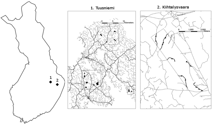
Fig. 1. The locations of the areas examined during the field inventories of unpaved forest road quality assessments. Both Tuusniemi and Kiihlelysvaara are located in the Finnish Lakeland region in Eastern Finland.
The field plots centres were selected to be respected to the whole road section. Their locations were logged by GPS receiver. Each plot was 10 metres long along the centreline of the road and varied in width with the width of the road and included side ditches and the status of the nearby vegetation too. Measurements of ruts and holes were carried out in these plots only. In order to avoid spatial accuracy problems of the centreline data to the ALS data, during the analysis the plots sizes were narrower than the road width. The area assessed included the road surface, shoulders and ditches (when present) and the roadside vegetation was assessed in 1 metre strips beyond the ditches or shoulders. No road maintenance had been carried out on these road sections at minimum for five years.
Following the quality standards for optimal forest road conditions developed by the Metsäteho organization (Korpilahti 2008), this study worked with the observations on structural condition, surface wear quality and flatness. The observations and measurements then were classified into one of three classes: good, satisfactory or poor. The classes are summarized in Table 1.
| Table 1. The road quality variables (structural condition, surface wearing and flatness) collected based on a Finnish Forest Road Quality recommendations (Korpilahti 2008) developed by Metsäteho Oy were classified to three quality categories in the study. The simplified table lists the road problems to be included in each category and the empirical assessment factors for good, satisfactory, and poor classes. | ||||
| Assessed roads quality variables | Road quality issues to pay attention while assessing each variable | Road quality classes | ||
| Good | Satisfactory | Poor | ||
| Structural condition | The whole road body condition. Visibility of driving lines. | The road surface is smooth; therefore, the driving speed does not need to be reduced | Some road quality problems (such as ruts) are visible, driving lines must be chosen with care and speeds have to be slightly reduced. | There are clearly visible ruts so the driving lines must be chosen carefully, and driving speeds have to be significantly reduced. |
| Surface wearing | The road wearing layer’s quality and material (fine, coarse, not present). | The road’s wearing layer is sufficiently thick and of good quality. | The wear layer is too thin, or the material is either too fine or too coarse. These are hindering vehicle movement and require slightly reduced speed. | The wear layer has majorly been worn away, or the material is too fine or too coarse. These factors are significantly hindering driving and speed reduction is necessary. |
| Flatness | The evenness of the road surface. Depressions, grooves and side bulges are present or not. Road drainage status. | The road has an even surface. There is no risk or damage to vehicles. The drainage of the surface is good. Road conditions will not hinder transportation or daily movement. | The wear layer is uneven, and the road has depressions, grooves and lateral bulges. There is visible damage. Lower speeds may be required in some places, but the risk of damage to a vehicle is quite small and will not hinder transportation or daily movement. | The road has depressions, grooves and lateral bulges, and/or drainage of its surface does not function well. The wear layer is defective, and driving conditions are obviously poor. It is necessary to reduce speed and to change the driving line frequently to avoid vehicle damage. The poor condition of the road hinders transportation and daily movement. |
Classifying the roads into good, satisfactory and poor quality can help decision makers to plan and schedule future road maintenance (Korpilahti 2008). Good quality roads do not require significant measures in the upcoming years, only basic maintenance. Satisfactory roads need follow-up and would benefit from targeted road improvements in addition to basic maintenance. Poor quality roads hinder transportation, and their conditions may further deteriorate, therefore urgent renovation is needed to reduce potential vehicle related damages, increase driving speed and driving times to save on transportation costs.
Poor quality roads were observed only during the second period of fieldwork (Table 2). The most frequent observation in both datasets was satisfactory quality, although poor quality with respect to surface wear was observed in six cases. The structural condition of the roads was the best: about two thirds of the observations being indicative of good quality and only three of poor structural condition.
| Table 2. Distribution of field observations between the road quality classes (poor, satisfactory and good) of road sections in two study areas. In Tuusniemi all 3 road quality classes were present, while in Kiihtelysvaara the road quality was better and only 2 classes were present. | ||||
| Tuusniemi, year 2014 | ||||
| Road quality class | Structural condition | Surface wearing | Flatness | Total number of road sections of each road quality class |
| Poor | 3 | 6 | 3 | 12 |
| Satisfactory | 13 | 27 | 22 | 62 |
| Good | 33 | 16 | 24 | 73 |
| Total number of road sections of each road quality parameter | 49 | 49 | 49 | 147 |
| Kiihtelysvaara, year 2013 | ||||
| Road quality class | Structural condition | Surface wearing | Flatness | Total number of road sections of each road quality class |
| Poor | 0 | 0 | 0 | 0 |
| Satisfactory | 3 | 7 | 6 | 16 |
| Good | 10 | 6 | 7 | 23 |
| Total number of road sections of each road quality parameter | 13 | 13 | 13 | 39 |
Carefully planned and constructed forest roads maintain better quality for a longer period (Forest practices code: forest road engineering guidebook 2002; Korpilahti 2008). The observations on three road quality variables (structural condition, flatness and surface wear quality) were recorded during the field work. The structural condition of a road depends on the road body. Well-constructed roads with a smooth surface may be said to be in good structural condition, but if the subgrade is not suitable, the road has a great deal of traffic on it or heavier vehicles use it than was expected, the surface may become damaged or rutted. In this case, it is necessary to drive carefully and reduce speed. Surface wear refers to the top layer of the road, that with which the vehicles make contact. The thickness of this layer is important, so that good wear means a thick, surface layer of good quality material. If it the material is too thin or too fine (satisfactory quality), it will soon be worn away (poor surface wear quality) and allow the other layers to be damaged. If a road is of good quality in terms of flatness, there will be hardly any inequalities observed on the surface, so that no speed reduction is needed and there is no risk of damage to the vehicle. The quality is satisfactory if the road has grooves and depressions, so that a reduction in speed is necessary and care has to be taken. If the road is in poor condition, bulges at its sides may affect the drainage system as well and depressions and grooves may hinder driving (Korpilahti 2008).
Data on the centrelines of the roads were available from the Finnish Transport Agency (2013) for both datasets.
2.2 Laser scanning data
The first area, Kiihtelysvaara, was scanned on 26 June 2009, providing high pulse density ALS data. An Optech ALTM Gemini laser scanning system was used from 600 m above ground level. The scanner had a field of view of 26° and a pulse repetition frequency of 100 kHz, which resulted in a sampling density of about 12 echoes received per square metre. The scanning strip had a width of approximately 320 m and 55% of side overlap. The four-year time gap between the field data and ALS data was acknowledged and will be discussed below.
The second area, Tuusniemi, was mapped between 23 and 30 July 2014 using a Leica ALS50-II laser scanning system from about 2000 m above ground level. The device had a 20° field of view, a 114 kHz pulse repetition frequency, and a 20% side overlap. The average sampling density was 1.1 pulses m–2.
2.3 Methodology
The ALS data were used in two steps so that the current paper introduces reference DEMs to increase the accuracy of the method described by Kiss et al. (2015) and test its applicability to a low pulse density dataset as well.
First, the reference DEM was created from the laser point cloud in the resolutions of 1 m and 2 m. Last and single echoes were used to create the terrain models with the following interpolation techniques: natural neighbour, spline, kriging, and inverse distance weighted. The reference DEM was used as a smooth road surface to reduce the topographic effect of the height differences in the roads on slopes. In order to reach this, the reference DEMs cell’s height values were reclassified: all reference DEM cells were reduced by the minimum value of the reference DEM in each assessed area.
Then we created the second set of DEMs (0.5 m and 1 m) with the interpolation as mentioned above to use them as input data for TPI and SE index calculation. For the calculations using reference DEMs, the reclassified values of the reference DEMs were extracted from the higher resolution DEMs before further calculations. The 1 m reference DEM was used for 0.5 m TPI and SE index calculations, and 2 m reference DEM was used for the 0.5 m TPI and SE calculations.
Secondly, we calculated TPI and SE. Furthermore, we calculated several ALS derived variables such as intensity of returns and height differences for the resolution 1 m and 0.5 m. Two surface quality indices were calculated: the Topographic Position Index (TPI) and the Standardized Elevation Index (SE) (Jenness Enterprises 2013). These were calculated for each cell in the DEM using a pre-defined neighbourhood size and shape of 3 m by 3 m rectangles. The TPI calculates the difference between the cell and the mean height of its neighbourhood, measured in the elevation units of the input data, e.g. in metres. Positive values mean a higher location than the neighbourhood, while negative values mean a lower location. The SE index calculates TPI divided by the standard deviation of the neighbourhood (Eqs. 1, 2). The SE index unit is in standard deviations.

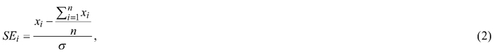
where:
xi = the height of the cell,
n = number of cells in the neighbourhood,
σ = standard deviation of height in the selected neighbourhood.
The variables for the predictions (Table 3) included TPI, SE surface quality indices and mean intensity values. The standard deviation and the mean values of the surface quality indices were assessed.
| Table 3. List of variables tested for prediction. In the table, dz: distance of height values from the reference DEM; dz5: distance of 5 random height values from the reference DEM SP: spline interpolation; KR: kriging interpolation; IDW: inverse distance-weighted interpolation; NN: natural neighbour interpolation. Topographic Position Indices (TPI) and Standardized Elevation (SE) names are the following: Interpolation Technique for Reference DEM ‘_’ Interpolation for Surface Quality Index. | ||
| ALS derived values – applied for height values in one cell | Reference DEM interpolation methods | Interpolation methods used for DEMs for TPI and SE calculations |
| intensity | SP | SP |
| range | KR | KR |
| variance | IDW | IDW |
| dz | NN | NN |
| dz^2 | ||
| dz^3 | ||
| dz5 | ||
| dz5 ^2 | ||
| mean (dz) | ||
| mean (dz^2) | ||
For the assessment of height values, we have used different threshold values. The distances were calculated only if they exceeded the threshold values; otherwise, they were assumed to be zero. A threshold of 20 cm was the highest, and we applied it when we aimed to identify poor quality roads only. While lower threshold values of 3 cm and 5 cm were tested for separating good quality roads.
Thirdly, several variables were used as predictors: TPI, SE, height distances between ALS ground points and the DEM. We calculated the difference between ALS hits and the reference DEMs. See Table 3 for the calculated variables. Then they were assessed by LDA to find out which of them describes the road quality classes the best. The predicted road quality variables were structural condition, surface wear and surface flatness. In the LDA, classification into three quality classes (poor, satisfactory, good) and two quality classes (poor versus non-poor, and good, versus non-good) were carried out.
The road quality classes were identified in one and two-step procedures as well. In the one-step classification, the road section samples were classified into one of the three quality classes (poor, satisfactory, good) at the same time. In order to improve the classification results, the classification was separated into two steps.
In the case of the low pulse density dataset, a two-step classification was applied. First, the good quality roads were identified from the data. Second, the poor quality ones were classified using different parameters. For the high pulse density data, only one step was used, as only two quality classes were involved. Fisher’s LDA, a supervised technique using quality information for classification purposes (Bishop 2006), was used here for dimension reduction before classification. LDA was used to determine variables for the three (poor, satisfactory, good) road quality classes in connection with the structural condition, surface wear and flatness. LDA was conducted in this analysis using the R package and leave-one-out evaluation. In the latter, the LDA was optimized once using leave-one-out cross-validation, and the same parameter was used in all the leave-one-out evaluations.
Finally, cross-validation was used to assess classification accuracy. The reliability of the classification was also discussed. Due to the low number of observations in the poor categories, leave-one-out cross-validation was chosen over training data. Cohen’s kappa values (Foody 2009) were calculated to assess the reliability of the classification, i.e. to measure the agreement between predicted classification and the field data. The test of differences was evaluated based on a confidence interval (CI) of 95% fitted to the estimated difference in the classification accuracy. McNemar’s test was run to assess marginal homogeneity. P-values were also calculated in relation to the classifications to assess whether there were any statistical differences between the road classes.
3 Results
3.1 High pulse density ALS dataset
The high and low pulse density ALS data showed different levels of accuracy in the quality classification as expected. The high pulse density data provided a better classification for the surface quality indices in all cases, for both the TPI and SE indices (Table 4).
| Table 4. Accuracy (%) of the classification of the TPI and SE index values for the structural condition assessments with and without a reference DEM. Kiihtelysvaara, high pulse density laser scanning data. Resolutions of 1 and 0.5 m. In the table, SP: spline interpolation; KR: kriging interpolation; IDW: inverse distance-weighted interpolation; NN: natural neighbour interpolation; TPI: Topographic Position Index; SE: Standardized Elevation Index. | ||||||
| Interpolation technique for surface index/reference DEM | No reference DEM | Reference DEM | ||||
| TPI index | SE index | TPI index | SE index | |||
| 1 m | 0.5 m | 1 m | 0.5 m | 0.5 m | 0.5 m | |
| IDW | 92% | 92% | 77% | 77% | 77% | 62% |
| KR | 69% | 92% | 46% | 62% | 77% | 54% |
| NN | 92% | 92% | 77% | 54% | 69% | 62% |
| SP | 62% | 77% | 62% | 77% | 85% | 54% |
Generating a reference DEM (Fig. 2) increased the accuracy of the classification, and the TPI index performed better than the SE index in this respect (Table 4). The SE index includes the standard deviation of the surrounding neighbourhood and introducing a smooth reference DEM reduced the elevation differences in the neighbourhood and improved the performance of the TPI index in the case of the kriging and natural neighbour interpolations. Variables other than the surface quality indices did not show any higher accuracy. The best results were also related to the structural condition. The precision of the classification was 77% using mean distance with spline and kriging interpolation of the reference DEMs. The results had the χ2 = 3 and p = 0.026 in McNemar’s test, and Cohen’s kappa values were close but less than 0.4, indicating only fair agreement. The use of a reference DEM increased the precision of the classification of the road sections only in a few cases in which high pulse density ALS data were used. We did not find correlation between intensity values and road quality.
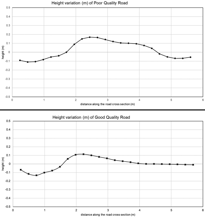
Fig. 2. Cross-sections of bad and good quality roads at 0.25 m resolutions. The Inverse Distance Weighted (IDW) interpolation technique was used to create the surfaces.
3.2 Low pulse density dataset
In order to analyse the low pulse density dataset, the road segments were classified in either one or two steps. In the one-step classification, all three quality classes (poor, satisfactory and good) were categorized at once, while the two-step classification was introduced to improve the accuracy of determining poor and good quality road sections, so that only the good quality classes were identified at first, and then the others.
A comparison of TPI indices between a good and a bad quality road with different interpolation techniques using a reference DEM with the low pulse density dataset is shown in Fig. 3. These cross sections are the same road profiles as in Fig. 4. The good quality road has close to zero TPI values after applying the reference DEM. The IDW interpolation has wider range of values along the cross-section, while the kriging interpolation smoothed the surface more, resulting in a smaller range of TPI values. In the case of a good quality road, the interpolation techniques gave similar results.
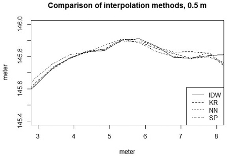
Fig. 3. The interpolation techniques at a resolution of 0.5 metre. In the figure, SP: spline interpolation; KR: kriging interpolation; IDW: inverse distance weighted interpolation; NN: natural neighbour interpolation.
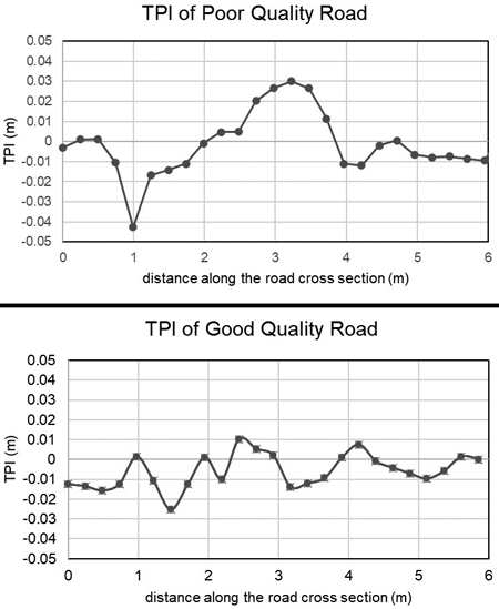
Fig. 4. TPI values for the cross-sections of a bad quality road (up) and good quality road (down). Different interpolations were used at a resolution of 0.25 m. Low pulse density dataset, Tuusniemi. In the figure TPI: Topographic Position Index.
The classification using the low-pulse density data with three quality classes performed worst in case of the separation of the satisfactory road category from the good and poor categories. On roads with smaller holes, surface inequalities cannot be distinguished and categorized well by low pulse density dataset. The classification results using only the surface quality indices showed low accuracy (Table 5). The best performance was obtained when spline interpolation was used for the reference DEM, as this classified the road quality correctly in 70–80% of cases. In the second step the satisfactory and good quality classes were merged and the poor quality class was treated separately. The classification accuracy increased when using only two quality classes (Table 5) as compared with the detection of three quality classes, because confusion of the satisfactory and good classes was avoided. The Kappa statistic was used to measure the accuracy with which the predicted classification agreed with the real situation and p-values were calculated to assess statistical significances of the differences between the categories. The classification of the surface wear quality data had kappa values between 0.2 and 0.4 in most cases, which means slight agreement with the assumption.
| Table 5. Classification accuracy (%) of TPI index values for structural condition assessments with the reference DEM interpolated with the indicated methods. Tuusniemi, high pulse density laser scanning data at a resolution of 0.5 m, verified against the field data. In the table, SP: spline interpolation; KR: kriging interpolation; IDW: inverse distance-weighted interpolation; NN: natural neighbour interpolation; TPI: Topographic Position Index. | ||||||
| Interpolation technique for reference DEM for TPI index | 3 quality classes | 2 quality classes (poor vs. non-poor) | p-value | |||
| Correctly classified roads | McNemar test (χ2) | Correctly classified roads | McNemar test (χ2) | |||
| IDW | IDW | 11% | 35.315 | 24% | 35.000 | <0.0001 |
| IDW | KR | 13% | 35.268 | 26% | 34.000 | <0.0001 |
| IDW | NN | 24% | 26.894 | 37% | 21.552 | <0.0001 |
| IDW | SP | 22% | 31.091 | 33% | 31.000 | <0.0001 |
| KR | IDW | 17% | 33.084 | 28% | 33.000 | <0.0001 |
| KR | KR | 20% | 32.084 | 30% | 32.000 | <0.0001 |
| KR | NN | 24% | 29.571 | 35% | 26.133 | <0.0001 |
| KR | SP | 7% | 35.121 | 28% | 33.000 | <0.0001 |
| NN | IDW | 17% | 33.084 | 28% | 33.000 | <0.0001 |
| NN | KR | 9% | 34.274 | 26% | 34.000 | <0.0001 |
| NN | NN | 26% | 25.256 | 57% | 16.200 | <0.0001 |
| NN | SP | 15% | 32.077 | 30% | 32.000 | <0.0001 |
| SP | IDW | 57% | 3.806 | 85% | 3.571 | 0.125 |
| SP | KR | 57% | 3.806 | 85% | 3.571 | 0.125 |
| SP | NN | 39% | 26.000 | 70% | 10.286 | 0.002 |
| SP | SP | 57% | 3.806 | 85% | 3.571 | 0.125 |
In order to improve performance, the classification was carried out using two-step classification. After the good quality roads were identified and separated from satisfactory and poor road, the 40 points belonging to satisfactory and poor roads were further analysed. The 40 observation points which were assessed are shown in Tables 5 and 6. The variables that performed best are shown with their class means and standard deviation. 78% of the good quality roads were identified correctly, and 75% of the roads classified as good were of good quality in the field observations.
| Table 6. Class means and standard deviations (SD) of the observations in each quality class for the variables which define good quality classes. In the table, dz: distance of height values from reference DEM; SP: spline interpolation; KR: kriging interpolation; IDW: inverse distance-weighted interpolation; NN: natural neighbour interpolation; TPI: Topographic Position Index. | |||||||||
| Variables | Interpolation technique | Poor class | Satisfactory class | Good class | p-value | McNemar test (χ2) | |||
| mean | SD | mean | SD | mean | SD | ||||
| (sum dz)^2 | SP | 149857.2 | 259466.2 | 49651.9 | 107136.8 | 49262.7 | 128945.5 | 0.887 | 6.444 |
| dz^2 | SP | 24978.0 | 43243.0 | 8786.3 | 18431.0 | 8044.1 | 19625.9 | 0.887 | 6.444 |
| dz | SP | 227.0 | 384.1 | 99.3 | 199.5 | 80.7 | 206.8 | 0.887 | 6.444 |
| mean (dz) | SP | 37.9 | 63.9 | 19.4 | 37.0 | 14.1 | 33.5 | 0.887 | 6.444 |
| mean (dz^2) | SP | 4163.3 | 7206.9 | 1749.2 | 3485.7 | 1332.2 | 3146.9 | 0.887 | 6.444 |
| (sum dz)^2 | NN | 0.1 | 0.2 | 17.6 | 42.1 | 47.2 | 229.0 | 0.887 | 6.444 |
| mean (dz) | NN | 0.0 | 0.1 | 0.0 | 0.1 | –0.1 | 0.3 | 0.669 | 1.145 |
| sum(dz)^2 | IDW | 0.0 | 0.0 | 0.2 | 0.4 | 85.9 | 471.2 | 0.669 | 1.145 |
| TPI using IDW | SP | 0.3 | 1.0 | 0.0 | 1.1 | –0.3 | 0.8 | 0.073 | 1.857 |
| TPI using KR | SP | 0.3 | 1.5 | –0.4 | 1.3 | –0.1 | 0.6 | 0.073 | 1.857 |
| TPI using SP | SP | 0.3 | 1.4 | –0.5 | 1.4 | –0.1 | 0.6 | 0.235 | 2.066 |
The other variant of two step classification was to first identify poor quality classes, and then do the classification to satisfactory and good classes. This gave a higher precision of finding only the poor quality classes than could be obtained with the whole dataset. In order to detect the road sections with the greatest height differences, the 20 cm threshold was used as described above. This successfully identified the two or three poor quality road sections using the 3 m and 20 m threshold for height differences. Spline interpolation was used for the reference DEM, and the TPI index at a resolution of 0.5 m with either the inverse distance-weighted, spline or kriging interpolation. The p-value of the McNemar index was between p = 0.0003 and p = 0.0005 in all 3 cases. The overall classification results (Table 7) show that the majority of the sites in the poor and good classes can be identified from the low pulse density laser datasets.
| Table 7. Forest road quality classification results of the analysed road sections using weighted distance from the Spline reference DEM with a 3 cm threshold and verified against field observations of structural condition. Overall accuracy: 62.5% Kappa = 0.214. | |||||
| Field measured classes | Classified as... | Classification overall | Producer accuracy (Precision) | ||
| Poor | Satisfactory | Good | |||
| Poor | 2 | 0 | 1 | 3 | 66.66% |
| Satisfactory | 2 | 2 | 5 | 9 | 22.22% |
| Good | 2 | 5 | 21 | 28 | 75.00% |
| Truth Overall | 6 | 7 | 27 | 40 | |
| User Accuracy | 33.33% | 28.57% | 77.77% | ||
The classification using the low pulse density dataset (Table 8) identified 21 out of the 28 good quality road sections, i.e. those not requiring any further action, and also 2 out of the 3 poor road sections which needed urgent maintenance. The remaining ones were considered uncertain and would require a field inventory to determine their exact condition. On the other hand, one of the three poor sections was identified as not requiring any action, even though maintenance was needed. The results show that ALS data can reduce the amount of fieldwork significantly.
| Table 8. Overall classification results for low resolution ALS area after the two-step identification of good and poor classes in terms of structural condition. Overall accuracy: 67.5% Kappa = 0.296 | |||||
| Field measured classes | Classified as... | Classification overall | Producer accuracy (Precision) | ||
| Poor | Satisfactory | Good | |||
| Poor | 2 | 0 | 1 | 3 | 66.66% |
| Satisfactory | 0 | 4 | 5 | 9 | 44.44% |
| Good | 0 | 7 | 21 | 28 | 75.00% |
| Truth Overall | 2 | 11 | 27 | 40 | |
| User Accuracy | 100.00% | 36.36% | 77.77% | ||
4 Discussion
A low (1.1 pulse m–2) and high pulse (12 pulses m–2) density laser scanning datasets were used to compare ALS derived features and their connection to three different road quality variables with and without the use of reference surfaces for road quality classification purposes. The introduction of references DEMs guaranteed a locally invariant analysis of road quality. The experimental areas were situated in Tuusniemi (low pulse density) and Kiihtelysvaara (high pulse density data), Finland. Two special indices at different resolutions and with different weighted variables, using four techniques for interpolating the reference DEM, were compared.
We note that the high pulse density airborne scanning data did not have any poor quality roads, only good and satisfactory ones, so that the two cannot be directly compared. The high pulse ALS data were obtained four years after the field data (13 plots), although both were recorded during a dry summer. The low pulse data was recorded in the same year and month as the field data (49 points) were collected. There were no signs of recent road maintenance, but the roads could have deteriorated during that interval, thus affecting the results of the classification. The low proportion of poor quality roads well represent the Finnish forest roads regarding quality. Determining satisfactory quality also leaves space for subjective judgement, as the guidelines for field inventories do not lay down exact figures for the allowable variation. Furthermore, the low pulse density dataset miss out information on holes or rocks in the roads.
Although the basic geometry of the road can be extracted from low pulse-density data as well (Craven and Wing 2014), the resolution achieved by ALS data is essential for any further analyses (White et al. 2010; Azizi et al. 2014). James et al. (2007) concluded that a density of 12 pulses m–2 was required to determine the depth of gullies, and our research supports this that high pulse dataset was required to distinguish more detailed road features, including ditches.
All the interpolation techniques performed well in creating a smooth surface for the reference DEM, but the choice of technique has to be made according to which achieves the best classification into satisfactory and bad quality roads. Road quality can be assessed through parameters such as weighted distances between height values and the reference DEMs and by using the TPI surface quality index with a spline interpolated reference DEM. The three categories chosen for evaluation, surface wear, flatness and structural condition, are closely related from the ALS point of view as well, as an inadequate surface wear layer and poor structural condition can detract from road flatness. As in the previous smaller dataset (Kiss et al. 2015), surface wear quality was derived with high precision, on the other hand the low pulse density dataset gave better results for structural condition using a reference DEM.
The best performance was obtained with the model that used the Topographic Position Index (TPI) with a reference DEM and a high pulse density dataset. The approach demonstrated here confirms that in the case of a low pulse density dataset the reference DEM improved the classification of the weighted variables (e.g. mean or average distances from the reference DEMs with suitable thresholds) when using a reference DEM. By contrast, the use of this approach with the TPI index did not give any significantly better classification results. The two-step classification provided the highest accuracy, with between 40% to 60% of the road sections classified with high precision as being of either good or poor quality, which after further improvements can reduce the amount of fieldwork required to assess the road quality on site. Low pulse density data can be used to derive the main road characteristics, but it is not sufficient to distinguish good roads from satisfactory ones.
The introduction of a reference DEM not only created a locally invariant analysis of road features but enabled the low pulse density dataset to identify the majority of poor and good quality roads with better success as well. Spline interpolation produced the best reference DEMs and lead to an up to 85% correct classification with the use of Topographic Position Index. The other variables were lower in accuracy. It is more important to have a denser point cloud or apply a reference DEM than to select an interpolation technique that yields high classification accuracy.
Identification of the worst and best quality roads can help in road maintenance to reduce the number of road sections which need to be checked in the field. The research tested how interpolation methods affect road quality indices and which performs best regarding TPI. The study can further be expanded by using car mounted LiDAR devices (Mobile Mapping 2020) to collect data alongside with the manual road check-ups.
5 Conclusions
In the case of the high pulse density dataset the introduction of a reference DEM did not significantly increase the performance of the interpolation methods. The TPI and SE indices calculated for higher resolution DEMs provided adequate information for classification purposes. The low pulse dataset performed better using the reference DEMs than without them. The use of the reference DEMs resulted in 75% of the good quality roads and 66% of the poor quality roads being correctly classified. The use of TPI index had an accuracy of 85%.
Declaration of openness of research materials, data, and code
The data, codes and other materials that support the findings of this study are available from the corresponding author, KW, upon reasonable request. We state that neither the study nor the analysis plan is preregistered.
Authors’ contributions
All authors contributed to the conception of research questions and design of the work. KW and JM collected the Kiihtelysvaara field data and KW, JM and TT collected the Tuusniemi field data. The analysis was carried out with all authors’ contributions. All authors participated in the interpretation of data and results, and writing.
Acknowledgements
We thank University of Eastern Finland for financing the research project, where this study was carried out. National Land Survey of Finland and the Finnish Transport Agency are also acknowledged for providing ALS data and road centrelines for the research.
Funding
The research was funded by the Doctoral Programme in Forests and Bioresources (FORES) at the University of Eastern Finland.
References
Azizi Z, Najafi A, Sadeghian S (2014) Forest road detection using LiDAR data. J For Res 25: 975−980. https://doi.org/10.1007/s11676-014-0544-0.
Barber D, Mills J, Smith VS (2008) Geometric validation of a ground-based mobile laser scanning system. ISPRS J Photogramm Remote Sens 63: 128–141. https://doi.org/10.1016/j.isprsjprs.2007.07.005.
Bater CW, Coops NC (2009) Evaluating error associated with lidar-derived DEM interpolation. Comput Geosci 35: 289–300. https://doi.org/10.1016/j.cageo.2008.09.001.
Bauwens S, Bartholomeus H, Calders K, Lejeune P (2016) Forest inventory with terrestrial LiDAR: a comparison of static and hand-held mobile laser scanning. Forests 7, article id 127. https://doi.org/10.3390/f7060127.
Beck SJC, Olsen MJ, Sessions J, Wing MG (2015) Automated extraction of forest road network geometry from aerial LiDAR. Eur J Forest Eng 1: 21–33. https://dergipark.org.tr/en/pub/ejfe/issue/5186/70456. Accessed 29 October 2020.
Bishop CM (2006) Pattern recognition and machine learning, information science and statistics. ISBN 0387310738. Springer-Verlag New York Inc., Secaucu, NJ, pp 186–195.
Buğday E (2018) Capabilities of using UAVs in forest road construction activities. Eur J Forest Eng 4: 56–62. https://doi.org/10.33904/ejfe.499784.
Clode S, Kootsookos P, Rottensteiner F (2004) The automatic extraction of roads from LiDAR data. In: Altan O (ed) Proceedings of the XXth ISPRS Congress Technical Commission III, 12–23 July 2004, Istanbul, Turkey. Int Arch Photogramm Remote Sens Spatial Inf Sci 35: 231–236. https://www.isprs.org/proceedings/XXXV/congress/comm3/papers/272.pdf.
Coulter ED, Sessions J, Wing MG (2006) Scheduling forest road maintenance using the analytic hierarchy process and heuristics. Silva Fenn 40: 143–160. https://doi.org/10.14214/sf.357.
Craven M, Wing M (2014) Applying airborne LiDAR for forested road geomatics. Scand J For Res 29: 174–182. https://doi.org/10.1080/02827581.2014.881546.
Finnish Transport Agency (2013) Digiroad – national road and street database. https://vayla.fi/en/transport-network/data/digiroad. Accessed 1 December 2020.
Foody GM (2009) Classification accuracy comparison: hypothesis tests and the use of confidence intervals in evaluations of differenc, equivalence and non-inferiority. Remote Sens Environ 113: 1658–1663. https://doi.org/10.1016/j.rse.2009.03.014.
Forest practices code: forest road engineering guidebook (2002) Ministry of Forests, British Columbia. https://www.for.gov.bc.ca/ftp/hfp/external/!publish/FPC%20archive/old%20web%20site%20contents/fpc/fpcguide/Road/FRE1.pdf. Accessed 3 July 2019.
James LA, Watson DG, Hansen WF (2007) Using LiDAR data to map gullies and headwater streams under forest canopy: South Carolina, USA. Catena 71: 132–144. https://doi.org/10.1016/j.catena.2006.10.010.
Jenness Enterprises (2013) Land facet corridor analysis. http://www.jennessent.com/arcgis/land_facets.htm. Accessed 2 February 2018.
Kiss K, Malinen J, Tokola T (2015) Forest road quality control using ALS data. Can J For Res 45: 1636–1642. https://doi.org/10.1139/cjfr-2015-0067.
Korpilahti A (ed) (2008) Metsäteiden kuntoinventoinnin ja kuntotiedon hyödyntämisen toimintamalli. [Operating model for forest road condition inventory and utilization of condition information]. Metsätehon raportti 202. http://www.metsateho.fi/wp-content/uploads/2015/02/Raportti_202_AK.pdf. Accessed 8 February 2018.
Lin Y, Hyyppä J, Jaakkola A (2011) Mini-UAV-borne LiDAR for fine-scale mapping. IEEE Geosci Remote S 8: 426–430. https://doi.org/10.1109/LGRS.2010.2079913.
Lloyd CD, Atkinson PM (2002) Deriving DSMs from LiDAR data with kriging. Int J Remote Sens 23: 2519–2524. https://doi.org/10.1080/01431160110097998.
Marinello F, Proto AR, Zimbalatti G, Pezzuolo A, Cavalli R, Grigolato S (2017) Determination of forest road surface roughness by kinect depth imaging. Ann For Res 60: 217–226. https://doi.org/10.15287/afr.2017.893.
Metsätilastollinen vuosikirja (2013) Skogsstatistisk årsbok. Finnish statistical yearbook of forestry. Official statistics of Finland: agricultur, forestry and fishery. Finnish Forest Research Institute (Metla), Vantaa. http://urn.fi/URN:ISBN:978-951-40-2449-8.
Mobile Mapping: Trimble Geospatial. https://geospatial.trimble.com/products-and-solutions/mobile-mapping-solutions. Accessed 6 November 2020.
Montealegre AL, Lamelas MT, De la Riva J (2015) Interpolation routines assessment in ALS-derived digital elevation models for forestry applications. Remote Sens 7: 8631–8654. https://doi.org/10.3390/rs70708631.
Piiparinen H (2003) Metsäteiden kunnossapitokustannukset Etelä-Suomen yksityismetsissä. [Forest road maintenance costs in private forests in Southern Finland]. Metsätieteen aikakauskirja 3/2003: 275–290. https://doi.org/10.14214/ma.6797.
Sibson R (1981) A brief description of natural neighbor interpolation. In: Barnett V (ed) Interpreting multivariate data. John Wiley & Son, New York, pp 21–36.
Smith PL (1979) Splines as a useful and convenient statistical tool. Am Stat 33: 57–62. https://doi.org/10.1080/00031305.1979.10482661.
Svenson G, Fjeld D (2016) The impact of road geometry and surface roughness on fuel consumption of logging trucks. Scand J For Res 31: 526–536. https://doi.org/10.1080/02827581.2015.1092574.
Talbot B, Pierzchała M, Astrup R (2017) Applications of remote and proximal sensing for improved precision in forest operations. Croat J For Eng 38: 1–10. http://www.crojfe.com/archive/volume-38-no.2/applications-of-remote-and-proximal-sensing-for-improved-precision-in-forest-operations/. Accessed 2 October 2020.
Tien D, Xiao Y, Qin Q-H (2008). A novel up-to-down algorithm for road extraction. Int J Tomogr Stat 9: 1–11. http://users.cecs.anu.edu.au/~Qinghua.Qin/publications/paper%20in%20book/pap-in-books-11.pdf. Accessed 2 March 2018.
Watson DF, Philip GM (1985) A refinement of inverse distance weighted interpolation. Geo-Processing 2: 315–327.
White RA, Dietterick BC, Mastin T, Strohman R (2010) Forest roads mapped using LiDAR in steep forested terrain. Remote Sens 2: 1120−1141. https://doi.org/10.3390/rs2041120.
Williams CKI (1998) Prediction with Gaussian processes: from linear regression to linear prediction and beyond. Learning in Graphical Models, Springer, Dordrecht, pp 599–621. https://doi.org/10.1007/978-94-011-5014-9_23.
Zhu L, Jaakkola A, Hyyppä J (2013) The use of mobile laser scanning data and Unmanned Aerial Vehicle images for 3D model reconstruction. Int Arch Photogramm Remote Sens Spatial Inf Sci XL-1/W2: 419–423. https://doi.org/10.5194/isprsarchives-XL-1-W2-419-2013.
Total of 33 references.
Send to email
