Ilkka Korpela  ,
Lauri Mehtätalo,
Lauri Markelin,
Anne Seppänen,
Annika Kangas
,
Lauri Mehtätalo,
Lauri Markelin,
Anne Seppänen,
Annika Kangas
Tree species identification in aerial image data using directional reflectance signatures
Korpela I., Mehtätalo L., Markelin L., Seppänen A., Kangas A. (2014). Tree species identification in aerial image data using directional reflectance signatures. Silva Fennica vol. 48 no. 3 article id 1087. https://doi.org/10.14214/sf.1087
Highlights
- Multispectral reflectance data showed a strong and spectrally correlated tree effect
- There was no gain in species classification from using species-specific differences of directional reflectance in real data and only a marginal improvement in simulated data
- The directional signatures extracted in multiple images are obscured by the intrinsic within-species variation, correlated observations and inherent reflectance calibration errors.
Abstract
Tree species identification using optical remote sensing is challenging. Modern digital photogrammetric cameras enable radiometrically quantitative remote sensing and the estimation of reflectance images, in which the observations depend largely on the reflectance properties of targets. Previous research has shown that there are species-specific differences in how the brightness observed changes when the viewing direction in an aerial image is altered. We investigated if accounting for such directional signatures enhances species classification, using atmospherically corrected, real and simulated multispectral Leica ADS40 line-camera data. Canopy in direct and diffuse illumination were differentiated and species-specific variance-covariance structures were analyzed in real reflectance data, using mixed-effects modeling. Species classification simulations aimed at elucidating the level of accuracy that can be achieved by using images of different quality, number and view-illumination geometry. In real data, a substantial variance component was explained by tree effect, which demonstrates that observations from a tree correlate between observation geometries as well as spectrally. Near-infrared band showed the strongest tree effect, while the directionality was weak in that band. The gain from directional signatures was insignificant in real data, while simulations showed a potential gain of 1–3 percentage points in species classification accuracy. The quality of reflectance calibration was found to be important as well as the image acquisition geometry. We conclude that increasing the number of image observations cancels out random observation noise and reflectance calibration errors, but fails to eliminate the tree effect and systematic calibration inaccuracy. Directional reflectance constitutes a marginal improvement in tree species classification.
Keywords
forestry;
reflectance calibration;
BRDF;
mixed-effects modeling;
Monte-Carlo simulation
-
Korpela,
Department of Forest Sciences, University of Helsinki, P.O. Box 27, FI-00014, Finland
E-mail
ilkka.korpela@helsinki.fi
- Mehtätalo, Faculty of Science and Forestry, University of Eastern Finland, P.O. Box 111, FI-80101 Joensuu, Finland E-mail lauri.mehtatalo@uef.fi
- Markelin, Department of Remote Sensing and Photogrammetry, Finnish Geodetic Institute, P.O. Box 15, FI-02431 Masala, Finland E-mail lauri.markelin@fgi.fi
- Seppänen, Faculty of Science and Forestry, University of Eastern Finland, P.O. Box 111, FI-80101 Joensuu, Finland E-mail anne.seppanen@arbonaut.com
- Kangas, Department of Forest Sciences, University of Helsinki, P.O. Box 27, FI-00014, Finland E-mail annika.kangas@helsinki.fi
Received 7 January 2014 Accepted 12 May 2014 Published 3 September 2014
Views 125614
Available at https://doi.org/10.14214/sf.1087 | Download PDF

1 Introduction
Information about the tree species is crucial on technical, economic and ecological grounds. However, species classification constitutes a challenge in passive optical remote sensing of forests – primarily because of small between-species differences in reflectance spectra, prominent within-species reflectance variation as well as within-image brightness trends caused by atmospheric effects and a changing view- and illumination geometry (Leckie et al. 2005). Because within-species reflectance variation is due to inherent target properties, probable advances in spectral species identification can be anticipated from enhanced observations and classification strategies. We discuss next the option of using radiometrically high-quality image observations and an original classification approach, in which species-specific differences in directional reflectance are exploited to enhance species identification.
Directional reflectance implies that the brightness of natural surfaces depends on the view- and illumination directions. This applies also to forest canopies, where the scattering of incoming light is volumetric (Kleman 1987; Deering et al. 1999). Directional reflectance is typically anisotropic and highly spectrally invariant. Hence, comparable directionality can be observed at different wavelengths. Directional reflectance is explained by shadow casting at different scales – at the canopy, crown, branch and needle levels (Li and Strahler 1986; Hapke et al. 1996). Strongest brightness trends occur, when the target, sensor and Sun are on the same (solar principal) plane. When they are collinear, the target is brightest, since shadows are occluded and backscattering dominates. Forward scattering (incl. glint) occurs, when the target is between the sensor and the Sun. Korpela et al. (2011) observed that directional effects, in Scots pine, Norway spruce and birch, are to some degree species- and wavelength-dependent. Neglecting the reality that accurate directional reflectance measurements are very difficult to attain, the proposal of utilizing directional reflectance in (tree species) classification is appealing, because it has not been reported in spite of ample coverage of the topic in remote sensing textbooks. However, the limitations of the required reflectance measurements warrant further discussion.
Recent advances in airborne photogrammetric camera data are of particular interest here. Namely, modern multispectral sensors are wide-band radiometers retaining the superior geometric accuracy of metric film cameras. The pixel values in absolutely calibrated sensors correspond to band-averaged at-sensor radiance (ASR) data (weighing by the bands’ spectral response functions), which are needed in the estimation of reflectance images. In that process, the radiance reflected towards the camera, right above the canopy, is inferred from the image ASR data that are measured through the atmosphere. Similarly, an estimate of the at-canopy solar illumination is derived using modeling. An ASR image has the so-called sensor-induced effects corrected, which include effects by shutter speed, optics, and f-number, inter alia. An accuracy of 5% is attainable (Dinguirard and Slater 1999; Ryan and Pagnutti 2009) and it also constitutes an upper limit of accuracy for any reflectance images. ASR images still exhibit ample scene-related variation that is not related to the reflectance properties of trees. The variation includes deviations in illumination, which comprises a complex wavelength-dependent angular distribution. The diffuse illumination component includes also the scattering and shading by close vegetation, in addition to landscape-level effects, such as those by near-by water bodies. The atmospheric effects are also directional. These scene-related sources of unwanted variation are accounted for in atmospheric correction, output of which are target reflectance images (e.g. Beisl et al. 2008). In aerial images, such data approximate (band-averaged) hemispherical-directional reflectance factors (HDRF), because the estimation of at-target diffuse illumination is always inaccurate. The lower the proportion of diffuse illumination, the better is the agreement of the target reflectance data with the optimal, but unattainable bi-directional reflectance quantities (Schaepman-Strub et al. 2006). Thus, any attempt to use aerial or satellite images for an exact measurement of target-specific, bi-directional reflectance properties will remain inexact. Bi-directional quantities can be accurately approximated, using laboratory measurements, in which both the incoming light and the viewing are highly directional (narrow cones).
Despite the aforementioned limitations of reflectance calibrated aerial images, we aimed to examine whether enhanced species classification is possible by accounting for the species-specific and wavelength-dependent directional reflectance differences. We used images, in which the sensor- and scene-related effects were minimized such that the image values link to the reflectance properties of trees. We applied both real and simulated data and developed a classifier that employs directional reflectance features. We examined the variance-covariance structures of real reflectance data, using mixed-effects modeling and used the results in simulations, which aimed at elucidating the influence of reflectance calibration errors and different observation geometries on tree species classification. We compared two classification approaches – the use of averaged image features against the utilization of directional signatures.
2 Materials and methods
In short, the experiment consisted of georeferenced trees that were visible in reflectance calibrated four-band aerial images (Sections 2.1 and 2.2). Tree crowns were modeled as opaque 3D surfaces and the image data for a tree were extracted for a sample of representative crown surface points. In that process, the camera-visible canopy, and pixels, were divided between sunlit and shaded illumination (Section 2.3). Each image observation was defined in a 2D view-illumination geometry, in which an average directional reflectance pattern was modeled for each tree species, image band and target illumination type (Section 2.4). Variance-covariance structures in reflectance data were analyzed, using mixed-effects models (Section 2.5). Tree species classifier that employs multispectral directional reflectance differences is presented in Section 2.6 and Section 2.7 explains the functioning of an image-based species classification simulator. The simulations applied different parameters for the number, geometry and quality of image observations and the resulting simulated data were classified by averaging or by accounting for the directional effects.
2.1 Field and image data
The experiment is in Hyytiälä, Finland (62°N, 24°E) and consists of 121 field plots and over 25 000 georeferenced trees, which were measured in 2005–2009, while the (ADS40) images were acquired in August 2008. Trees were positioned with an accuracy of 0.1–0.3 m in x and y, using a total station or a photogrammetric-geodetic method (Korpela et al. 2007). The crown status and treetop position were updated to 2008, using visual interpretation of high-resolution images and airborne LiDAR data, which could be superimposed in the images to support crown detection. Most intermediate and nearly all suppressed trees were occluded in all views and rejected from analyses. Treetop positioning methods were forward ray intersection and monoplotting, which was needed for trees that were visible in only one image. In it, the operator pointed the treetop in the image, casting down an image ray (cylinder) that intersected the LiDAR point cloud. The tree set consisted of 15 188 dominant–intermediate trees (height 2–38 m, age 15–150 yrs, Table 1).
| Table 1. Mean and sdev (standard deviation, in parentheses) of stem diameter (d1.3), height (h), crown diameter (dcr), and age. | |||
| Variable | Pine N = 5914 | Spruce N = 7105 | Birch N = 2169 |
| d1.3, cm | 20.1 (6.5) | 20.3 (7.9) | 15.1 (6.7) |
| h, m | 17.5 (4.1) | 18.1 (5.8) | 16.4 (5.3) |
| dcr, m | 2.8 (0.9) | 2.9 (0.9) | 2.6 (0.9) |
| Age, years | 59.5 (25.3) | 66.4 (28.7) | 47.0 (24.6) |
The images were acquired with the Leica ADS40 line sensor that hosts CCD lines on the focal plane (Fricker and Hughes 2004). It is shutter-free and provides ‘continuous’ imaging. Each CCD line has 12 000 pixels and the lines are oriented in the across-track direction with offsets in the along-track direction. So-called nadir lines (N00) are close to the optical axis and view the scene below (Fig. 1). Viewing in forward and backward directions is accomplished by lines with offsets in these directions. The same target may thus be recorded several times and different targets that map to the same pixel position are seen in a fixed projection and illumination across the entire image (Fig. 1). We used four-color image data, which are provided by two sets of four-line assemblies. They provide stereo data with 16° angular offset, in the nadir (N00) and backward directions (B16). Both assemblies host a CCD line for the blue (BLU), green (GRN), red (RED) and near-infrared (NIR) bands, which are 50 nm wide and centered at wavelengths of 465, 555, 653 and 860 nm. The image acquisition took two hours, using an airplane with a ground speed of 60–70 m/s. The solar elevation increased from 27 to 37° and isolated clouds resulted in disqualified observations. The ground resolution was 10–40 cm for the flying heights of 1–4 km. There were 15 strips and 19 four-color (N00 or B16) images with reference trees (Table 2). Natural and artificial reference targets were measured for nadir reflectance spectra during the image acquisition (Markelin 2010).
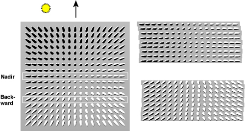
Fig. 1. Illustration of perspective imaging of a ‘forest scene’. A frame camera image on the left has white rectangles depicting the nadir- and backward viewing lines of the ADS40. Sections of the nadir (N00) and backward viewing (B16) images are shown on the right. The flying direction is upwards and it is 25° off with respect to the direction to the Sun.
| Table 2. Characteristics of the ADS40 data acquisition by each four-color image. ‘Trees lost’ is the percentage of trees occluded or shaded by clouds in the image coverage. | ||||||||
| Flying altitude [km] | Start time [GMT] | Flight path azimuth [°] | Sun azimuth [°] | Sun elevation [°] | Tree observations | Trees lost [%] | Integration time [ms] | Active CCD lines |
| 1 | 0656 | 349 | 119.3 | 27.1 | 48 | - | 1.94 | N00 |
| 1 | 0703 | 169 | 121.0 | 27.8 | 6345 | 8 | 1.94 | N00 |
| 1 | 0711 | 349 | 123.1 | 28.6 | 9027 | 24 | 1.94 | N00 |
| 1 | 0718 | 169 | 124.9 | 29.3 | - | - | 1.94 | N00 |
| 1 | 0725 | 349 | 126.7 | 30.0 | 6867 | - | 1.94 | N00 |
| 1 | 0733 | 169 | 128.8 | 30.7 | 6917 | - | 1.94 | B16 |
| 2 | 0745 | 349 | 132.0 | 31.8 | 8844 | 3 | 2.77 | N00 |
| 2 | 0753 | 169 | 134.2 | 32.5 | 11332 | 8 | 2.77 | N00 |
| 2 | 0800 | 349 | 136.1 | 33.1 | 7550 | 17 | 2.77 | B16 |
| 2 | 0808 | 169 | 138.3 | 33.7 | 11077 | 5 | 2.77 | B16 |
| 3 | 0818 | 349 | 141.1 | 34.4 | 13571 | 2 | 4.16 | N00 |
| 3 | 0818 | 349 | 141.1 | 34.4 | 14876 | 0 | 4.16 | B16 |
| 3 | 0825 | 169 | 143.1 | 35.0 | 12045 | 16 | 4.16 | N00 |
| 3 | 0825 | 169 | 143.1 | 35.0 | 11280 | 8 | 4.16 | B16 |
| 3 | 0833 | 260 | 145.4 | 35.5 | 8742 | 28 | 4.16 | N00 |
| 3 | 0833 | 260 | 145.4 | 35.5 | 9694 | 35 | 4.16 | B16 |
| 4 | 0843 | 169 | 148.3 | 36.1 | 13531 | 4 | 5.54 | N00 |
| 4 | 0843 | 169 | 148.3 | 36.1 | 12073 | 0 | 5.54 | B16 |
| 4 | 0852 | 260 | 151.0 | 36.7 | 12352 | 6 | 5.54 | N00 |
| 4 | 0852 | 260 | 151.0 | 36.7 | 12941 | 11 | 5.54 | B16 |
2.2 Geometric and radiometric image post-processing
Owing to the ‘continuous exposure’, the position and attitude of the ADS40 were determined with satellite positioning and inertial measurements. These were refined in aerial triangulation to sub-pixel accuracy. Each image line had a unique perspective projection for the 12 000 pixels. We implemented an iterative procedure for the object-space → image-space -transformation to enable the retrieval of pixel data for the reference trees.
At-sensor radiance images were input to the estimation of atmospherically corrected reflectance images, using the Leica XPro 4.2 software. The images, consisting of 'target reflectance values' (Beisl et al. 2008) were considered as approximations of HDRF data (Schaepman-Strub et al. 2006; Heikkinen et al. 2011). Henceforth, because the very exact algorithm of XPro remained unknown, we use the general terms R data and R images for the atmospherically corrected ADS40 images. Markelin et al. (2010) analyzed the accuracy of the R data and reported relative RMS accuracies of 5% for NIR, 7–12% for RED and GRN, and up to 20% for BLU.
2.3 Assigning reference trees with spectral R (reflectance) data
The next step was to assign pixel values to each tree and derive spectral mean features for the BLU, GRN, RED and NIR bands in two classes of illumination, the sunlit and shaded canopy. Because of the large number of trees and images, the procedure was automated. The canopy geometry was modeled, using LiDAR data. The crowns were approximated by opaque and convex surfaces of revolution, which were fitted to LiDAR data using non-linear regression. (Fig. 2, Korpela et al. 2011). The pixel data were next sampled for 121 crown surface points. Besides the treetop, there were ten layers with twelve points at 30° intervals, reaching down to the 60% relative height. Each point was tested for shading and occlusion, using the surrounding LiDAR points, which were treated as 0.7-m-wide spheres. A ray was cast towards Sun and the sensor and tested for intersection. If free from obscuring canopy (incl. the tree itself), the point was classified as sunlit and camera-visible. Pixel data were retrieved for camera-visible points only and duplicate pixels were omitted. The illumination classes were sunlit (Su), self-shaded (Se), neighbor-shaded, neighbor- and self-shaded (Fig. 2).
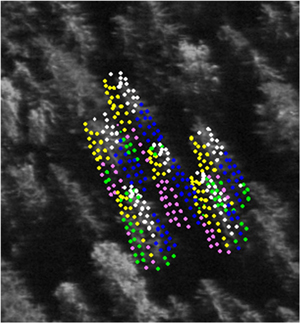
Fig. 2. Illustration of sidelit spruce crowns that were sampled for image data in a 1-km B16 BLU image. Points not self-occluded were superimposed. Colors depict the assigned illumination class: white = sunlit (Su), yellow = self-shaded (Se), blue = neighbor-shaded, magenta = neighbor- and self-shaded. Green points are occluded by a neighboring tree.
The eight-term feature vector consisted of the mean R of the four bands in the sunlit (Su) and self-shaded (Se) illumination. Table 3 lists the mean R values. Trees are dark in BLU-RED, while scattering is stronger in NIR. Relative between-species differences are small, being 2–30% in the Su class. The differences between the Su and Se classes were smaller than expected considering the proportion of diffuse illumination, which was from approximately 25 to 1% for wavelengths of 400 to 800 nm (Iqbal 1983). The illumination classes were clearly averaged, but the relative R differences were logical, being from 8% in BLU (high proportion of diffuse light) to 28% in NIR. Contrast was largest in birch, which has larger and more round crowns.
| Table 3. Mean reflectance factors of pine, spruce and birch crowns at nadir. BLU (blue), GRN (green), RED (red), NIR (near-infrared). Se = self-shaded, Su = sunlit illumination class. | ||||
| Illumination – Species | BLU | GRN | RED | NIR |
| Se – Pine | 0.037 | 0.041 | 0.030 | 0.169 |
| Se – Spruce | 0.035 | 0.035 | 0.024 | 0.155 |
| Se – Birch | 0.038 | 0.044 | 0.031 | 0.227 |
| Su – Pine | 0.040 | 0.051 | 0.037 | 0.220 |
| Su – Spruce | 0.038 | 0.047 | 0.032 | 0.224 |
| Su – Birch | 0.042 | 0.060 | 0.043 | 0.322 |
2.4 View-illumination observation geometry
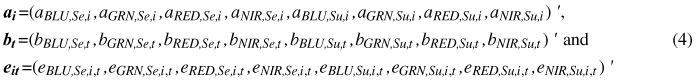
The view-illumination geometry of each image observation (tree in an image) was characterized by relative azimuth (ϕ) and view zenith (θview) angles. ϕ is 0° for perfectly front-lit trees seen in the in backscattering geometry and ±180° for back-lit trees in forward scattering geometry. We assumed azimuth symmetry and ϕ ∈ [0°,180°]. θview in the ADS40 data was 0–35°. Finally, the geometry was defined in a polar representation (Eq. 1, Fig. 3).
![]()
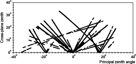
Fig. 3. Distribution of all image observations in the xy view-illumination geometry (Eq. 1). The x coordinate is negative in the forward-scattering geometry (back-lit trees dominate) and positive in the backscattering geometry, in which front-lit trees dominate the view.
Fig. 3 illustrates the geometry of all observations. The ‘V-shaped’ patterns that meet at the nadir (x = 0°, y = 0°) are observations in the N00 images, while the rest are B16 observations. The most horizontal patterns with small y values are from two E⇔W-oriented strips, in which image lines were almost collinear with the solar azimuth direction. This is the geometry of prominent directional effects. The two sloping patterns in Fig. 3 resulted from the B16 images of the same strips 0833 and 0852 (Table 2). The ‘images’ in Fig. 1 were acquired by flying 25° off with respect to the direction to the Sun, which gives an ϕ of 115° and 65° for the N00 image observations. In Fig. 3, these data would create a steep V-shaped pattern, while the B16 image observations would shown an L-shaped pattern through points (0, 34°), (18°, 0°), and (26°, 22°).
2.5 Analyzes of reflectance variance using mixed-effects modeling
Ideally, accurate reflectance calibration results in R data that are free from all scene-related effects. Yet, when limiting to a single species, such R data show random between-tree variation that is due to differences in crown structure, adjacency effects in NIR, and measurement errors, which combine of many sources including errors in mapping 3D points to the right pixels, in the determination of illumination and occlusion and in the geometry of the crown models. Systematic within-image trends are primarily due to the species-specific directional reflectance, but may include compound effects, for example due to the varying background effects in different azimuth directions (Fig. 1). It is clear that due to incorrect reflectance calibration, real R data also include residue scene-related variation, which is systematic in nature.
We used mixed-effects modeling to examine the variance-covariance structures in the R feature data. The general form of the linear model (for some combination of species and image feature) is given in Eq. 2. The first term describes the aforementioned within-image trends and comprises polynomial models of directional reflectance anisotropy (Fig. 4) by Korpela et al. (2011) that were re-estimated here The tree effect is supported by the idea that the crown structure and local scattering influence the observed reflectance in all view geometries. Systematic measurement errors can also contribute to this term, for example those caused by an erroneous crown model. The image effect considers between-image offsets in reflectance calibration. It could also be xy-dependent, because the atmospheric effects are azimuthally asymmetric (Privette and Vermote 2004). The residual term combines the unexplained variance. The modeling is explained in more detail in the remaining part of this Section.
![]()
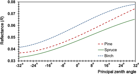
Fig. 4. Examples of directional R anisotropy models for the GRN band in the Su illumination class showing the response along the solar principal plane (y = 0°). The principal plane (view) zenith angle ranges from –32° (forward scattering) to +32 (backscattering), i.e. from back-lit to front-lit trees. The R of pine deviates somewhat from spruce and birch as a function of the view zenith angle, which constitutes the directional ‘signature’.
Because there were four bands and two illumination classes, a system of mixed-effect models was specified. In Eq. 3, t refers to a tree, and i refers to an image, and the fixed part f (x, y; α) specifies the systematic dependence on the xy geometry, using a polynomial surface with a species-band-illumination -specific parameter vector α. The R variation for a given species, for each combination of band and illumination, was modeled, using a system of eight models:
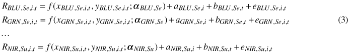
The random part includes a random image effect a, tree effect b and residual e, which are all independent, zero-mean normally distributed random variables with constant variances. The tree effects are common for all observations of the same tree in different images, and they specify the average difference of the tree in question from the average tree. The variance of tree effect explains how much of the variation left unexplained by f (x, y; α) due to the tree being similar in different views. The image effects are common for all trees of the same image, and they specify the average difference of the image in question from an average image. Their variance shows the variation between images. As stated, we hypothesized that the image effects are mostly related to the image-specific atmospheric correction, whereas the tree effects are related to tree-specific reflectance properties (structure). The residual includes the variation, which cannot be explained by the fixed part, image effect, and tree effect. The eight models were estimated separately for all three tree species, leading to a total of 24 models (one model for each cell of Table 3).
For a given tree species, the eight random effects and error terms of the models are correlated. That is, the random effects for a given tree or image are likely to be similar for all eight band–illumination -specific models. This correlation was estimated, using the predicted values of the random effects and residuals. We first extracted the predicted tree effects, image effects, and residuals for each tree, image and tree within image, respectively, as
Then we computed the empirical variance-covariance matrices A8×8 = var(ai), B8×8 = var(bt) and R8×8 = var(eit). These matrices were computed separately for each of the three tree species.
2.6 Classification of tree species with single and multi-image observations
We compared two classification scenarios. The first used averaged spectral eight-term R feature vectors (cf. Packalén et al. 2009) and quadratic discriminant analysis (QDA, Hastie et al. 2001). This scenario was applied for both single and multi-image data, and due to the parametric nature of the QDA, directional effects can have a major influence on the performance. The second classifier was applied in multi-image data and it made use of the directional R anisotropy differences (Fig. 4), which were described by the f (x, y; α) polynomials of Eq. 3. A tree observed in N images results in N observation vectors consisting of the mean values of BLU, GRN, RED, NIR in the Su and Se illumination classes. The expected R = f (x, y; α) values for the three species are contrasted with the N observation vectors resulting in N difference vectors. Mahalanobis distance is computed for each. The needed 8 × 8 covariance matrix is constant and it was estimated from a sample over all real data. The Mahalanobis distances per species are summed and the classification result is defined by the minimum. The algorithm bears resemblance to discriminant analysis, except that the class-specific mean vectors vary with the view-illumination geometry (Fig. 4). Overall classification accuracy, the simple Kappa and the producer accuracy at the species level were the performance measures.
2.7 Simulator for spectral tree species classification
In short, a Monte-Carlo simulator was used to create synthetic R data, using different values for strip overlap, solar azimuth difference and reflectance calibration accuracy. These tree-level data were then classified, using the two methods of Section 2.6. Strip overlap affects the view geometry and number of observations per tree, azimuth difference influences view-illumination geometry, and reflectance calibration accuracy defines the radiometric quality of the R data.
A simulation consists of 100 imaging campaigns, each of which has eight parallel N⇔S-oriented ADS40 strips resulting in a block of 16 images. A mixed forest is created for each campaign and each tree of known species is checked for inclusion in the images and the corresponding xy. The expected values of spectral R features for a tree are simulated, using f (x, y; α) of Eq. 3. Multivariate error terms are simulated after that. We used the mvn(mean, cov) function in the R-environment (Venables and Ripley 2002; package ‘mclust’ by Fraley et al. 2012) to create realizations of multinormal distributions. Tree effects were given by mvn(0, A) and the same eight-term vector was added to all realizations of the same tree. Residual vectors by mvn(0, R) were added for each simulated tree and image combination. The image effect, i.e. the reflectance calibration errors were simulated as relative errors. Their variance-covariance structure and dependency on the xy view-illumination geometry were altered to simulate different scenarios of R calibration accuracy. The observations combining the anisotropy, tree effect and the residual term were multiplied by a coefficient cf, which was band- and image-specific (Eq. 5). Errors made in the estimation of the atmospheric status are correlated in the visible range bands (Privette and Vermote 2004) and are likely also correlated temporally, within a photogrammetric image block that covers a restricted area.
We chose a simple model to derive the coefficients, which allows the relative errors to depend on the view-illumination xy-geometry.
![]()
The expectance of cf and a0 is 1, while E(a1) = E(a2) = 0. The parameters a0, a1, and a2 were drawn from multinormal distributions by first assuming the variance of a0 for BLU. The variance of cf was assumed to be lower in GRN, RED and NIR, in that order as indicated by results in Markelin et al. (2012).
3 Results of experiments
3.1 Mixed-effects modeling of the real R (reflectance) data
Table 4 shows the relative division of R variance according to Eq. 3. The directional R anisotropy explained up to 45% of the total variance in BLU, while it was 18–42% in GRN and RED, and only 7% in NIR. In diffuse illumination, 8–36% of the total variance was explained by the species-specific reflectance anisotropy in BLU, GRN and RED. The effect was strongest in BLU. Essentially, there was no directionality in diffuse NIR illumination.
| Table 4. Partition of reflectance factor (R) variance between the terms of the mixed-effects models (Eq. 3). Percentages (%) of total R variance. Su refers to the directly illuminated canopy and Se to self-shaded canopy in diffuse illumination. BLU (blue), GRN (green), RED (red), NIR (near-infrared). | ||||||||
| Band | BLU | GRN | RED | NIR | ||||
| Illumination | Su | Se | Su | Se | Su | Se | Su | Se |
| Directional anisotropy | ||||||||
| Pine | 51 | 36 | 41 | 19 | 42 | 15 | 4 | 1 |
| Spruce | 43 | 21 | 36 | 10 | 37 | 10 | 13 | 0 |
| Birch | 41 | 29 | 20 | 9 | 18 | 8 | 4 | 0 |
| Mean | 45 | 29 | 32 | 13 | 33 | 11 | 7 | 0 |
| Tree effect | ||||||||
| Pine | 13 | 12 | 35 | 38 | 35 | 41 | 58 | 60 |
| Spruce | 14 | 13 | 39 | 42 | 37 | 42 | 58 | 67 |
| Birch | 26 | 15 | 54 | 44 | 55 | 44 | 70 | 65 |
| Mean | 18 | 13 | 43 | 41 | 42 | 42 | 62 | 64 |
| Image effect | ||||||||
| Pine | 28 | 42 | 6 | 14 | 5 | 11 | 9 | 2 |
| Spruce | 33 | 54 | 5 | 17 | 5 | 15 | 3 | 1 |
| Birch | 20 | 41 | 3 | 10 | 3 | 9 | 6 | 2 |
| Mean | 27 | 46 | 5 | 14 | 4 | 12 | 6 | 2 |
| Residual | ||||||||
| Pine | 8 | 10 | 18 | 29 | 18 | 33 | 29 | 37 |
| Spruce | 10 | 12 | 21 | 30 | 21 | 32 | 26 | 32 |
| Birch | 13 | 15 | 22 | 38 | 23 | 39 | 20 | 33 |
| Mean | 10 | 13 | 20 | 32 | 21 | 35 | 25 | 34 |
As much as 64% and 62% of the R variance in NIR was explained by the tree effect in diffuse and direct illumination, respectively. The differences were small between illumination classes on all bands. In NIR, both the reflectance and transmittance are high resulting in strong first- and second-order scattering. The tree structure influences the signal more in NIR compared to the visible range. Atmospheric effects are also minor in NIR. The fact that the BLU band showed the highest values for anisotropy and lowest for the tree effect is explained by the diffuse nature of the BLU illumination. However, errors in atmospheric correction can show as compound effects, because the image effect (Eq. 3) omitted xy dependencies and considered only between-image offsets. The image effect explained 20–54% of the R variance in the BLU band. The proportions were higher in diffuse illumination, i.e. in ‘darker’ objects, which is logical.
3.2 Species classification in real ADS40 R (reflectance) data
3.2.1 Classification using averaged and nadir-corrected R features in single image data
We first tested with single image data by applying different training–validation scenarios. In addition to the eight mean R features, we applied a ‘normalization to nadir’, using general anisotropy polynomials, which were obtained by fitting Eq. 3 to data combining all species. The Rnadir values were derived by subtracting the xy dependent part of the polynomials from the observed R. Training sets had 300 randomly selected trees per species. Table 5 shows results for tests, in which the training and validation data were from the same image. Table 6 has results for tests, in which the B16 and N00 images from the same strip were used for training and validation. The nadir correction improved performance in only one case, which probably was due to between-image errors in reflectance calibration. And, as could be expected, the performance deteriorated when the training and validation data were from different images, i.e. view-illumination (xy) geometries.
| Table 5. Classification performance when the training and validation data were from the same image. The sdevs of the overall accuracy values varied from 0.4 to 0.7% in 100 trials with randomized training data. | ||||||
| Image | Height, km | Accuracy % | Kappa | Pine % | Spruce % | Birch % |
| 0753_N00 | 2 | 78.7 | 0.657 | 80.6 | 78.2 | 75.9 |
| 0808_B16 | 2 | 80.4 | 0.683 | 84.0 | 79.5 | 73.7 |
| 0818_N00 | 3 | 75.6 | 0.604 | 75.5 | 76.4 | 73.5 |
| 0825_N00 | 3 | 74.3 | 0.582 | 75.8 | 74.2 | 70.0 |
| 0833_N00 | 3 | 75.7 | 0.610 | 74.9 | 77.0 | 73.6 |
| 0843_N00 | 4 | 77.8 | 0.641 | 80.7 | 76.9 | 72.8 |
| Table 6. QDA classification performance when the training and validation data were from different 3 km images in the same strip. Tests with nadir normalized (Rnadir, *) data are included. | ||||||
| Training | Validation | Accuracy % | Kappa | Pine | Spruce | Birch |
| 0818_B16 | 0818_N00 | 66.3 | 0.480 | 73.6 | 56.7 | 77.2 |
| * | * | 69.6 | 0.510 | 64.6 | 74.2 | 68.3 |
| 0825_B16 | 0825_N00 | 62.8 | 0.386 | 38.6 | 83.7 | 66.5 |
| * | * | 58.2 | 0.341 | 58.9 | 54.0 | 70.4 |
| 0833_B16 | 0833_N00 | 72.5 | 0.575 | 80.4 | 64.8 | 78.6 |
| * | * | 70.4 | 0.540 | 75.6 | 65.4 | 74.5 |
3.2.2 Classification using averaged and nadir-corrected R features in multi-image data
A straightforward way to combine several image observations per tree is to compute average feature vectors (Packalén et al. 2009). Using data comprising all images (results not tabulated) and 3 × 300 trees for training the QDA, the classification accuracy was 80.7% (κ = 0.69). Restricting to the 2–4-km images and to the 3–4-km images, the accuracies were 79.5% and 79.2%, respectively. With six and four images in the 3 and 4 km data, accuracies were 76.7% and 79.4%. Almost similar classification accuracy was reached, using single image data (Table 5). When the training and validation sets were split between strips, the accuracy again deteriorated. For example, using two images in strips 0818 and 0825 for training and validation, resulted in an accuracy of 34%, which improved to 54%, using nadir-normalized Rnadir data.
3.2.3 Classification utilizing directional R (reflectance) signatures in multi-image data
When all images were combined, there were trees with up to 15 observations. Using the classifier and the directional image features explained in Section 2.6, the accuracy was 78.2%, and it improved to 78.4%, when between-image R offsets were calibrated, using 3×100 trees as radiometric signals. Confining to ten 3–4-km images, the mean classification accuracy was 78.2%, which is 1% lower compared to the use of QDA and averaged features. The accuracy improved one percentage point to 79.2% when R offsets were corrected with 3×100 trees that were visible in all images. In 3-km images, the classification accuracy was 76.8%, which is the same as with averaged features.
The results are disappointing as the accuracy did not improve compared to the use of averaged features. The R differences are not strong (Fig. 4), and the data was undoubtedly affected by calibration errors, which we tried to correct, using trees as calibration targets. Calibration errors were analyzed by Markelin et al. (2012), using the laboratory-measured reflectance tarps, and the RMS-% values were 5–35% in BLU, GRN and RED, and 5–10% in NIR. The optimality of our classifier can also be questioned.
3.3 Results of simulations in multi-image data
3.3.1 Classification utilizing directional R anisotropy
In each simulation, there were 8000–12 000 trees in the ‘forest’ and 100 'imaging campaigns'. Each campaign comprised eight N⇔S-oriented strips. The overlaps were 35 or 67%, which gave on average 2.9 or 4.7 observations per tree, respectively. The mean ϕSun were 90°, 135° or 180°, and deviated ±25º in each simulated campaign. The nadir image lines sampled along the solar principle plane, when ϕSun was 90°, which is the geometry of strongest the directional effects. Fig. 5 illustrates the xy observation geometry for a campaign, in which the nadir image lines viewed all trees as ‘side-lit’, because ϕSun was 140°–161°.
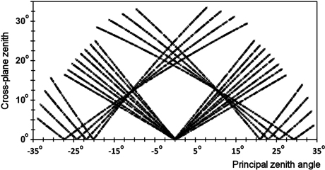
Fig. 5. xy observation geometry (Eq. 1) of eight N⇔S-oriented strips and 16 images. ϕSun changed from 140 to 161° with 3° intervals. The V- and L-shaped patterns represent observations in the nadir and backward viewing images, respectively.
R calibration accuracy was simulated at plausible and very accurate levels (Table 7). As each campaign consisted of eight strips, there were in total 16 four-band images and 16×4×3 model (image×band×{a0, a1, a2}) parameters (Eq. 5) to be simulated. We assumed poorest relative R calibration accuracy in the BLU band. The sdev (standard deviation) of a1 was larger than sdev of a2 indicating that error trends are stronger in the direction of the solar principal plane. When simulating the plausible accuracy scenario, the parameters for the offset and trends in Eq. 5 had positive correlation (r = 0.8) between bands, but within one band they were simulated with r = 0.0, which may be unrealistic. The between-image correlations were positive, r = 0.7 across bands and r = 0.8 for observations on the same band.
| Table 7. Sdevs of the parameters of the reflectance calibration error functions (Eq. 5, parameters a0, a1, a2). Plausible and accurate level of errors. x ∈ [–0.6, 0.6] and y ∈ [0, 0.6] in radians. BLU (blue), GRN (green), RED (red), NIR (near-infrared). | ||||
| BLU | GRN | RED | NIR | |
| a0 | 0.20 | 0.10 | 0.10 | 0.075 |
| a1 | 0.05 | 0.025 | 0.025 | 0.020 |
| a2 | 0.025 | 0.0125 | 0.0125 | 0.010 |
| a0 | 0.05 | 0.03 | 0.02 | 0.02 |
| a1 | 0.01 | 0.005 | 0.005 | 0.005 |
| a2 | 0.005 | 0.005 | 0.005 | 0.0025 |
Left columns of Table 8 show the results for the plausible accuracy scenario. The classification accuracy was 75–87% for trees observed in 2.9 or 4.7 images. To compare, the accuracy was 76.8% with 4.8 observations in real 3-km data. The strip overlap and the solar azimuth difference influenced the performance (accuracy of (a & b) > (c & d) > (e & f) in Table 8). Accuracies of up to 90% (κ ~ 0.86) were obtained for trees observed in 6 images. In practice, it must be noted that only the tallest are visible at high view zenith angles. The CVs of per species κ and accuracy were higher compared to the CVs of the overall accuracy. This was due to the correlated calibration errors – the accuracy of the 'brightest' or 'darkest' species could deteriorate in all images of a campaign. CVs were largest, when the azimuth difference was smallest (e & f in Table 8), because the directional signatures were smallest in this geometry and the classification performance was more sensitive to R calibration errors.
| Table 8. Classification performance in simulations using plausible and very accurate R calibration accuracy and directional signatures. Simulated strips were flown in N⇔S direction. Values in parentheses are CVs (%). Strip overlaps were 35% or 67% and the mean ϕSun were 90°, 135° or 180° resulting in six view-illumination geometry scenarios. In each scenario, the first line shows the results for all trees (2.9 or 4.7 image observations per tree), while the next lines show the results for trees observed in 2, 4 or 6 images. | ||||||||||
| N | Plausible reflectance calibration accuracy | Very accurate reflectance calibration | ||||||||
| Accuracy | Kappa | Pine | Spruce | Birch | Accuracy | Kappa | Pine | Spruce | Birch | |
| a) 35% overlap, solar azimuth 90 (strong directional effects) | ||||||||||
| 2.9 | 79 (5) | 0.68 (8) | 82 (11) | 77 (11) | 77 (10) | 83 (1) | 0.74 (2) | 87 (3) | 80 (4) | 80 (3) |
| 2 | 69 (6) | 0.53 (11) | 72 (22) | 67 (23) | 68 (12) | 74 (2) | 0.60 (4) | 80 (6) | 69 (9) | 72 (5) |
| 4 | 91 (5) | 0.87 (7) | 95 (4) | 90 (6) | 89 (9) | 94 (1) | 0.91 (2) | 97 (2) | 94 (2) | 91 (2) |
| b) 67% overlap, solar azimuth 90° | ||||||||||
| 4.7 | 87 (4) | 0.80 (7) | 91 (7) | 86 (7) | 84 (9) | 89 (1) | 0.84 (2) | 93 (2) | 88 (3) | 87 (3) |
| 2 | 79 (9) | 0.68 (15) | 82 (15) | 77 (17) | 77 (15) | 83 (4) | 0.75 (7) | 89 (6) | 79 (9) | 82 (8) |
| 4 | 80 (7) | 0.71 (12) | 84 (16) | 78 (16) | 79 (13) | 84 (4) | 0.76 (7) | 89 (6) | 82 (9) | 82 (8) |
| 6 | 91 (3) | 0.87 (5) | 95 (4) | 91 (5) | 88 (8) | 93 (1) | 0.89 (2) | 96 (2) | 93 (3) | 90 (3) |
| c) 35% overlap, solar azimuth 135 (intermediate directional effects) | ||||||||||
| 2.9 | 78 (6) | 0.67 (11) | 82 (14) | 76 (13) | 76 (10) | 83 (1) | 0.74 (2) | 88 (3) | 80 (4) | 80 (3) |
| 2 | 69 (7) | 0.54 (14) | 74 (20) | 66 (21) | 68 (13) | 74 (2) | 0.62 (4) | 81 (5) | 70 (8) | 72 (5) |
| 4 | 89 (6) | 0.84 (9) | 92 (10) | 88 (7) | 87 (8) | 94 (1) | 0.90 (2) | 96 (2) | 94 (2) | 91 (3) |
| d) 67% overlap, solar azimuth 135° | ||||||||||
| 4.7 | 84 (4) | 0.77 (7) | 89 (11) | 82 (12) | 82 (9) | 89 (2) | 0.83 (2) | 93 (3) | 87 (4) | 86 (4) |
| 2 | 71 (11) | 0.57 (22) | 77 (33) | 67 (37) | 71 (17) | 80 (5) | 0.70 (8) | 86 (10) | 77 (11) | 76 (8) |
| 4 | 83 (6) | 0.74 (10) | 87 (11) | 80 (14) | 81 (13) | 87 (4) | 0.80 (6) | 92 (5) | 84 (8) | 84 (7) |
| 6 | 89 (4) | 0.84 (6) | 93 (8) | 88 (9) | 87 (8) | 92 (2) | 0.88 (2) | 96 (2) | 92 (3) | 89 (4) |
| e) 35% overlap, solar azimuth 180° (mild directional effects) | ||||||||||
| 2.9 | 75 (10) | 0.62 (18) | 78 (24) | 72 (21) | 74 (10) | 83 (2) | 0.75 (3) | 89 (4) | 82 (5) | 79 (3) |
| 2 | 70 (9) | 0.55 (16) | 75 (18) | 65 (18) | 69 (12) | 77 (2) | 0.65 (4) | 84 (5) | 74 (7) | 73 (5) |
| 4 | 81 (13) | 0.71 (22) | 81 (33) | 81 (26) | 81 (11) | 91 (2) | 0.87 (3) | 95 (4) | 92 (4) | 86 (3) |
| f) 67% overlap, solar azimuth 180° | ||||||||||
| 4.7 | 77 (11) | 0.66 (20) | 78 (35) | 78 (23) | 76 (10) | 87 (2) | 0.80 (3) | 92 (5) | 86 (5) | 82 (3) |
| 2 | 68 (16) | 0.52 (31) | 71 (44) | 67 (40) | 69 (20) | 81 (4) | 0.71 (7) | 87 (10) | 78 (12) | 77 (8) |
| 4 | 76 (10) | 0.64 (18) | 79 (31) | 76 (24) | 73 (14) | 84 (4) | 0.76 (7) | 91 (7) | 83 (9) | 79 (9) |
| 6 | 81 (12) | 0.71 (20) | 80 (34) | 82 (21) | 80 (9) | 89 (2) | 0.84 (3) | 95 (4) | 89 (5) | 84 (4) |
Simulations were done next assuming an exceedingly correct R calibration (Table 8). The sdevs of the parameters defining the relative R calibration error were reduced notably (Table 7). The correlations of errors between bands and images were reduced (r = 0.5) to increase randomness in Eq. 5. The relative calibration errors were approximately 5, 3, 2, and 2%, for the BLU, GRN, RED, and NIR bands, respectively. This level of accuracy is difficult to attain even with high-grade field spectrometers. As expected, the performance improved and the CVs of κ decreased compared to the plausible R calibration accuracy scenario. Owing to the improved radiometric quality, the influence of azimuth difference was significantly lower. The best-case accuracy was 92–94% for trees with 4–6 image observations across a wide range of xy-geometries (Table 8).
3.3.2 Classification utilizing averaged spectral features
We further classified the simulated multi-image data with QDA, using an averaged eight-term feature vector [RBLU,Su, RGRN,Su, RRED,Su, RNIR,Su, RBLU,Se, RGRN,Se, RRED,Se, RNIR,Se]. The training data consisted of 160 trees per species. The best performance was associated with the geometry that minimizes the directional effects (ϕSun ~180°). The classification accuracy was 85.4% (κ = 0.781) when the training data were representative of all images and the R calibration accuracy was plausible (f in Table 9). Then again, best-case accuracy was 87%, using directional R signatures (b in Table 8). The gain from directional signatures was thus low, 1–2 percentage points, being slightly higher with very accurate R calibration. The calibration accuracy had almost no effect in the QDA classification owing to the use of averaged features. The representativeness of the training data was important (results not tabulated) as with real line-sensor data.
| Table 9. QDA classification performance in simulations using averaged R features and the same simulated data (a through f) as in Table 8. Values in parentheses are CVs (%). Plausible (Pl) and accurate (vA) reflectance calibration accuracy. Strip overlaps (O-%) were 35% or 67%, giving on average 2.9 or 4.7 image observations per tree. | ||||||||
| Case | Overlap, % | mean ϕsun | R calibration | Accuracy | Kappa | Pine | Spruce | Birch |
| a | 35 | 90° | Pl | 78.5 (1.0) | 0.677 (1.7) | 84.6 (2) | 74.8 (3) | 76.1 (2) |
| vA | 79.5 (0.8) | 0.693 (1.4) | 84.5 (2) | 76.1 (2) | 77.9 (2) | |||
| b | 67 | 90° | Pl | 82.7 (1.1) | 0.741 (1.9) | 88.3 (2) | 79.7 (3) | 80.1 (2) |
| vA | 83.1 (0.8) | 0.747 (1.4) | 88.5 (2) | 80.5 (3) | 80.5 (2) | |||
| c | 35 | 135° | Pl | 79.1 (0.9) | 0.686 (1.6) | 83.7 (2) | 75.4 (3) | 78.2 (2) |
| vA | 80.2 (0.8) | 0.703 (1.3) | 84.0 (2) | 76.6 (2) | 79.9 (2) | |||
| d | 67 | 135° | Pl | 83.3 (1.2) | 0.749 (1.9) | 86.9 (2) | 80.2 (2) | 82.7 (2) |
| vA | 84.3 (0.8) | 0.764 (1.3) | 87.2 (2) | 81.7 (2) | 83.9 (2) | |||
| e | 35 | 180° | Pl | 82.1 (1.1) | 0.732 (1.9) | 84.4 (2) | 79.0 (2) | 83.0 (2) |
| vA | 83.5 (0.8) | 0.753 (1.4) | 85.3 (2) | 80.3 (2) | 84.9 (2) | |||
| f | 67 | 180° | Pl | 85.4 (1.2) | 0.781 (2.0) | 87.7 (2) | 82.4 (2) | 86.1 (2) |
| vA | 86.5 (0.8) | 0.797 (1.4) | 88.5 (2) | 83.6 (2) | 87.3 (1) | |||
4 Discussion
4.1 Limitations of the study
We next draw attention to potential weaknesses in our experiment. The image acquisition was non-optimal, because it consisted of several acquisition heights and the flight line directions were not altered systematically. The reflectance calibration of the images was made with the Leica XPro only, using plausible assumptions about the atmospheric status. Despite careful experimentation, geometric errors influenced image orientation parameters (sub-pixel level), treetop position estimates (0.1–0.3 m), crown models (smooth rotation-symmetric opaque surfaces vs. complex semi-transparent volume) and the canopy geometry, which was represented by LiDAR data. The errors and simplifying assumptions explain in part why the reflectance values between sunlit and self-shaded illumination classes differed less than 30%. Directional reflectance is a property of a surface. Here it was a property of an object, the camera-visible tree crown in two illumination classes. The sunlit and shaded 'crown patches' were different in every image, and the observed directional reflectance was undoubtedly influenced by geometric errors. For comparison, directionality is less ambiguous in satellite images, in which a pixel can represent tens of tree crowns, which demonstrate a 'surface' in that scale.
Our directional R observations with the ADS40 undoubtedly deviate from helicopter measurements using a spectroradiometer (Kleman 1987). The R data were in agreement with existing measurements for pine, spruce and birch (Jääskeläinen et al. 1994), except for a difference of about 20% in the BLU band, which was also observed for the radiometric reference targets (Markelin et al. 2010). Thus, it is probable that the R values in BLU were systematically too high and showed a large between-image variation. Dalponte et al. (2013) report R values, which were 200–250% times higher than in our data. They used a hyperspectral sensor that viewed Scots pine and Norway spruce trees in the nadir.
4.2 Sources of reflectance (R) variation in aerial image data
As much as 58–70% of the R variance in NIR was due to the tree effect, while directional R anisotropy explained only 4–14%. The tree effect was also substantial and spectrally correlated in the visible range bands and it was consistently largest in birch, which differs in structure from the two conifers examined. Then again, directional anisotropy explained less of the R variance in birch. Birch crowns are more round in shape and the foliage is concentrated on the ‘crown envelope’, which affects shadow casting.
The consequence from the prominent and spectrally correlated tree effect is that additional image observations will reduce observation noise, but species classification accuracy will improve only modestly.
The tree effect was lesser in the BLU band. Korpela et al. (2011) showed that the relative brightness difference (with respect to solar azimuth) within crowns was modest in BLU, which is explained by the substantial atmospheric scattering that contributes to the pixel values. Because trees are dark in BLU, the contrast is diminished by the path radiance. Atmospheric correction cannot restore local contrast. Because of the path radiance and errors in atmospheric correction, and other possible compound effects, the results were likely biased in BLU.
4.3 Usability of directional reflectance anisotropy in spectral tree species classification
Regarding our main aim, there basically was no gain from applying the directional reflectance signatures in the real ADS40 data. The identified causes were the marginal between-species differences in reflectance and the remnant reflectance calibration errors. The simulated gain was 1–3 percentage points in overall classification accuracy, compared to the use of averaged features and the QDA classifier, which was trained with training data representing all images. We simulated scenarios illustrating both very accurate and plausible R calibration accuracy and even the plausible scenario was probably optimistic, because the simulated data met the normality assumptions and sampled the entire view-illumination space. We tried to correct the remnant calibration errors in real data, using trees that were visible to several images, but the improvement in classification performance was marginal.
The image feature comprised of mean BLU, GRN, RED and NIR values sampled from the camera-visible crown, which was divided between sun-lit and self-shaded parts. As such, the division between direct and diffuse illumination improves species classification performance (Korpela 2004; Larsen 2007). In practice, however, there are trees that remain occluded in some images, or trees that are in diffuse illumination. Similarly, trees observed near the solar principal plane at high view zenith angles, can only be viewed for the front-lit or back-lit crown. In real data, missing observations will reduce classification accuracy, which therefore will be highest for the tallest camera-visible trees. The number of image observations always improved the accuracy in simulations.
The optimal flying direction of a line sensor was found to depend on the classification strategy. The use of directional signatures is optimal if the image lines are aligned with the solar azimuth, while the use of averaged spectral features is optimal, when the image lines are in perpendicular configuration.
Our classifier could potentially be improved, especially, if high-quality reflectance anisotropy models would exist for the target classes (cf. Deering et al. 1999). More complex covariance structures could in such case be incorporated to enhance the classification. Using the same Hyytiälä ADS40 data, Heikkinen et al. (2011) combined the data by the nadir (N00) and backward (B16) viewing sensor lines in a non-parametric (SVM) classification algorithm and obtained classification accuracies of up to 88%, when restricting to a single image strip. Owing to ample training data, the SVM algorithm learned the directional effects in the N00 and B16 spectral features. However, the results were poor, when the SVM model was validated in a different pair of N00 and B16 R images.
4.4 Practical implications and suggestions for future research
As such, deficits of our experiment warrant further research in the usability of directional reflectance signatures. However, our results strongly imply that the gain in species identification performance will be low, even if the reflectance calibration of images is accurate. Thus, it may be reasonable to state that reflectance calibration of aerial images is not worth striving for. At-sensor radiance (ASR) images, in which the sensor-induced effects (e.g. shutter speed, f-number) are accounted for, demonstrate stable radiometry if the scene illumination and atmospheric status remain unchanged (e.g. Dalponte et al. 2013, 2014). However, an extensive imaging campaign can take several hours, and the time between overlapping flight lines and images can be substantial. Thus, the ASR images will show temporal (spatial) trends and addition to the directional within-image trends. Spectral features that are extracted from images of a large image block become inconsistent, which has been an overlooked issue in empirical tree species classification studies, because of the small number of images and test sites. The consistency can be improved by reflectance calibration or by means of flight planning.
Species classification by means of cost-efficient remote sensing remains a bottleneck, despite promising results with very dense airborne LiDAR data (Holmgren et al. 2008; Korpela et al. 2010). We anticipate that a strong tree effect will also be observed in NIR LiDAR data, as there is no shading (or illumination classes) due to the constant back-scattering geometry. The tree effect in LiDAR data (of particular type) will therefore better display the between-tree variation in crown structure.
The potential of ADS40 sensors in tree species classification can be improved by an additional band in the red-edge, λ = 700 nm (Heikkinen et al. 2010; Pant et al. 2013). The most recent version of the ADS40 is a three-line four-band sensor. Thus, advances in photogrammetric sensors can be anticipated as well as those in hyperspectral (HS) imaging, which was studied in Norway by Dalponte et al. (2013), using a VIS-NIR range sensor. Species classification accuracy was 89% for four classes, using 52 narrow bands (λ = 410–845 nm). Their results apply to near-nadir geometry and a manual delineation of pixels. At the imaging height of 1.5 km the pixel size was 52 × 40 cm and the image was 640 m wide. A reduction from 160 to 52 bands did not influence the classification (SVM) performance. Tests using smaller feature sets were not reported, however this constitutes an interesting research question. Pant et al. (2013) showed that an optimized five-band (wide-band) sensor provides stand-level data that result in comparable classification performance with a HS sensor. The geometry is a particular issue in HS imaging, because the exterior orientation is exclusively dependent on direct georeferencing, and the interior orientation (passage of image rays from the projection center to the pixels of different bands) is not as accurate as in photogrammetric sensors. Thus, there can be mismatch between the HS and other data, which may hinder automatic analyses and data fusion (e.g. Dalponte et al. 2013, 2014; Pant et al. 2013).
We used spectral mean values for each tree as classification features. Other features may well be more characteristic of tree species. These include higher moments, spectral indices and transformations, within-crown brightness trends and the image texture, which is potentially available in high-resolution images. Due to perspective mapping, even such features will likely display directional effects.
We examined species classification of individual trees, which was feasible because the slow manual tree detection was accurate. Automated detection methods will likely be less accurate. Our approach of mapping crown points to images is feasible in the commonly applied area-based forest inventory methods, which combine sparse LiDAR data with aerial images (Packalén et al. 2009) or utilize images only (Straub et al. 2013). A detailed canopy model is required for the estimation of illumination conditions and camera-visibility.
5 Conclusions
The use of between-species differences in directional reflectance anisotropy does not constitute a significant improvement to tree species classification, when using multispectral aerial images, even if the reflectance calibration of the images is very accurate. This was obvious in both real and simulated data. A strong spectrally correlated tree effect was observed implying that the relative brightness of a tree is very similar in all view directions and across the multispectral bands.
Acknowledgements
We would like thank Dr. Ulrich Beisl for his valuable criticism as well as those by the peer reviewers. Finding by the Academy of Finland, TEKES, University of Helsinki, University of Eastern Finland and Suomen Luonnonvarojen tutkimussäätiö since 2008 have facilitated this research.
References
Beisl U. (2012). Reflectance calibration scheme for airborne frame camera images. International Archives of the Photogrammetry, Remote Sensing and Spatial Information Sciences 39 (Part B7): 1–7.
Beisl U., Telaar J., Schönermark M.V. (2008). Atmospheric correction, reflectance calibration and BRDF correction for ADS40 image data. International Archives of the Photogrammetry, Remote Sensing and Spatial Information Sciences 37 (Part B7): 7–12.
Dalponte M., Ørka H.O., Gobakken T., Gianelle D., Næsset E. (2013). Tree species classification in boreal forests with hyperspectral data. IEEE Transactions on Geoscience and Remote Sensing 51(5): 2632–2645. http://dx.doi.org/10.1109/TGRS.2012.2216272.
Dalponte M., Ørka H.O., Ene L.T., Gobakken T., Næsset E. (2014). Tree crown delineation and tree species classification in boreal forests using hyperspectral and ALS data. Remote Sensing of Environment 140: 306–317. http://dx.doi.org/10.1016/j.rse.2013.09.006.
Deering D.W., Eck T.F., Banerjee B. (1999). Characterization of the reflectance anisotropy of three boreal forest canopies in spring-summer. Remote Sensing of Environment 67(2): 205–229. http://dx.doi.org/10.1016/S0034-4257(98)00087-X.
Dinguirard M., Slater P.N. (1999). Calibration of space-multispectral imaging sensors: a review. Remote Sensing of Environment 68(3): 194–205. http://dx.doi.org/10.1016/S0034-4257(98)00111-4.
Fraley C., Raftery A., Scrucca L. (2012). Package ‘mclust’. http://cran.r-project.org/web/packages/mclust/mclust.pdf. [Cited 15 Sept 2012].
Fricker P., Hughes D. (2004). ADS40 – a BRDF research tool. In: Schönermark M., Geiger B., Röser H.P. (eds.). Reflection properties of vegetation and soil – with a BRDF data base. Wissenschaft und Teknik Verlag, Berlin. p. 337–347. ISBN 3-89685-565-4.
Hapke B., DiMucci D., Nelson R., Smythe W. (1996). The cause of the hot spot in vegetation canopies and soils: shadow-hiding versus coherent backscatter. Remote Sensing of Environment 58(1): 63–68. http://dx.doi.org/10.1016/0034-4257(95)00257-X.
Hastie T., Tibshirani R., Friedman J. (2001). The elements of statistical learning: data mining, inference and prediction. Springer-Verlag, New York. 745 p.
Heikkinen V., Tokola T., Parkkinen J., Korpela I., Jääskeläinen T. (2010). Simulated multispectral imagery for tree species classification using support vector machines. IEEE Transactions on Geoscience and Remote Sensing 48(3): 1355–1364. http://dx.doi.org/10.1109/TGRS.2009.2032239.
Heikkinen V., Korpela I., Honkavaara E., Parkkinen J., Tokola T. (2011). An SVM classification of tree species radiometric signatures based on the Leica ADS40 sensor. IEEE Transactions on Geoscience and Remote Sensing 49(11): 4539–4551. http://dx.doi.org/10.1109/TGRS.2011.2141143.
Holmgren J., Persson Å., Söderman U. (2008). Species identification of individual trees by combining high resolution LiDAR data with multi-spectral images. International Journal of Remote Sensing 29(5): 1537–1552. http://dx.doi.org/10.1080/01431160701736471.
Iqbal M. (1983). An introduction to solar radiation. Academic Press. 389 p. ISBN 0-12-373752-4.
Jääskeläinen T., Silvennoinen R., Hiltunen J., Parkkinen J. (1994). Classification of the reflectance spectra of pine, spruce, and birch. Applied Optics 33(12): 2356–2362.
Kleman J. (1987). Directional reflectance factor distributions for two forest canopies. Remote Sensing of Environment 23(1): 83–96. http://dx.doi.org/10.1016/0034-4257(87)90072-1.
Korpela I. (2004). Individual tree measurements by means of digital aerial photogrammetry. Silva Fennica Monographs 3. 93 p.
Korpela I. (2007). 3D treetop positioning by multiple image matching of aerial images in a 3D search volume bounded by lidar surface models. Photogrammetrie, Fernerkundung, Geoinformation 1/2007: 35–44.
Korpela I., Tuomola T., Välimäki E. (2007). Mapping forest plots: an efficient method combining photogrammetry and field triangulation. Silva Fennica 41(3): 457–469. http://dx.doi.org/10.14214/sf.283.
Korpela I., Ørka H.O., Maltamo M., Tokola T., Hyyppä J. (2010). Tree species classification using airborne LiDAR – effects of stand and tree parameters, downsizing of training set, intensity normalization, and sensor type. Silva Fennica 44(2): 319–339. http://dx.doi.org/10.14214/sf.156.
Korpela I., Heikkinen V., Honkavaara E., Rohrbach F., Tokola T. (2011). Variation and directional anisotropy of reflectance at the crown scale – implications for tree species classification in digital aerial images. Remote Sensing of Environment 115: 2062–2074. http://dx.doi.org/10.1016/j.rse.2011.04.008.
Larsen M. (2007). Single tree species classification with a hypothetical multi-spectral satellite. Remote Sensing of Environment 110(4): 523–532. http://dx.doi.org/10.1016/j.rse.2007.02.030.
Leckie D.G., Tinis S., Nelson T., Burnett C., Gougeon F.A., Cloney E., Paradine D. (2005). Issues in species classification of trees in old growth conifer stands. Canadian Journal of Remote Sensing 31(2): 175–190.
Li X., Strahler A.H. (1986). Geometric-optical bi-directional reflectance modeling of a coniferous forest canopy. IEEE Transactions on Geoscience and Remote Sensing 24(6): 281–293. http://dx.doi.org/10.1109/TGRS.1986.289706.
Markelin L., Honkavaara E., Beisl U., Korpela I. (2010). Validation of the radiometric processing chain of the Leica airborne photogrammetric sensor. International Archives of the Photogrammetry, Remote Sensing and Spatial Information Sciences 37 (Part 7A): 145–150.
Markelin L., Honkavaara E., Schläpfer D., Bovet S., Korpela I. (2012). Assessment of radiometric correction methods for ADS40 imagery. Photogrammetrie, Fernerkundung, Geoinformation 3/2012: 251–266.
Packalén P., Suvanto A., Maltamo M. (2009). A two stage method to estimate species-specific growing stock. Photogrammetric Engineering and Remote Sensing 75(12): 1451–1460.
Pant P., Heikkinen V., Hovi A., Korpela I., Hauta-Kasari M., Tokola T. (2013). Evaluation of simulated bands in airborne optical sensors for tree species identification, Remote Sensing of Environment 138: 27–37. http://dx.doi.org/10.1016/j.rse.2013.07.016.
Privette J., Vermote E. (2004).The impact of atmospheric effects on directional reflectance measurements. In: Schönermark M., Geiger B., Röser H.P. (eds.). Reflection properties of vegetation and soil – with a BRDF data base. Wissenschaft und Teknik Verlag, Berlin. p. 225–242. ISBN 3-89685-565-4.
Ryan R.E., Pagnutti M. (2009). Enhanced absolute and relative radiometric calibration for digital aerial cameras. In: Fritsch D. (ed.). Photogrammetric week 2009. WichmannVerlag, Heidelberg, Germany. http://www.ifp.uni-stuttgart.de/publications/phowo09/index.en.html.
Schaepman-Strub G., Schaepman M.E., Painter T.H., Dangel S., Martonchik J.V. (2006). Reflectance quantities in optical remote sensing – definitions and case studies. Remote Sensing of Environment 103(1): 27–42. http://dx.doi.org/10.1016/j.rse.2006.03.002.
Straub C., Stepper C., Seitz R., Waser L.T. (2013). Potential of UltraCamX stereo images for estimating timber volume and basal area at the plot level in mixed European forests. Canadian Journal of Forest Research 43: 731–741. http://dx.doi.org/10.1139/cjfr-2013-0125.
Venables W.N., Ripley B.D. (2002). Modern applied statistics with S. Fourth edition. Springer, New York. 495 p.
Total of 33 references
