Ilari Lehtonen  ,
Petri Hoppula,
Pentti Pirinen,
Hilppa Gregow
,
Petri Hoppula,
Pentti Pirinen,
Hilppa Gregow
Modelling crown snow loads in Finland: a comparison of two methods
Lehtonen I., Hoppula P., Pirinen P., Gregow H. (2014). Modelling crown snow loads in Finland: a comparison of two methods. Silva Fennica vol. 48 no. 3 article id 1120. https://doi.org/10.14214/sf.1120
Highlights
- A new method to model crown snow loads is presented and compared with a previously published simpler method
- The heaviest crown snow loads in Finland are found to typically occur in the eastern parts of the country
- The relative importance of different snow load types varies between different regions of Finland.
Abstract
The spatial occurrence of heavy crown snow loads in Finland between 1961 and 2010 is studied by using for the first time a model that classifies the snow load into four different types: rime, dry snow, wet snow and frozen snow. In producing this climatology, we used meteorological observations made at 29 locations across Finland. The model performance is evaluated against classified daily images of canopy snow cover and with the help of two short case studies. The results are further compared to those achieved with a simpler method used in previous studies. The heaviest crown snow loads are found to occur typically in eastern Finland. The new method reveals that this holds not only for the total snow loads but also for the different snow load types, although there are certain differences in their geographical occurrence. The greatest benefit achieved with the new method is the inclusion of rime accretion. The forests most prone to heavy riming are those located on tree-covered hills in northern Finland, but as the terrain elevation affects riming efficiency greatly, these small-scale variations in the snow load amounts could not be described in this study in great detail. Moreover, the results are more inaccurate in northern Finland where variations in the terrain elevation are greater than elsewhere. Otherwise, the largest uncertainties in this study are related to wind speed measurements and possibly partly because of that, we were not able to detect any significant trends in the crown snow-load amounts over the study period.
Keywords
climate;
forests;
snow damage;
rime;
dry snow;
wet snow;
frozen snow
-
Lehtonen,
Finnish Meteorological Institute, P.O. Box 503, FI-00101 Helsinki, Finland
E-mail
ilari.lehtonen@fmi.fi
- Hoppula, Finnish Meteorological Institute, P.O. Box 503, FI-00101 Helsinki, Finland E-mail petri.hoppula@fmi.fi
- Pirinen, Finnish Meteorological Institute, P.O. Box 503, FI-00101 Helsinki, Finland E-mail pentti.pirinen@fmi.fi
- Gregow, Finnish Meteorological Institute, P.O. Box 503, FI-00101 Helsinki, Finland E-mail hilppa.gregow@fmi.fi
Received 18 February 2014 Accepted 16 June 2014 Published 30 July 2014
Views 239937
Available at https://doi.org/10.14214/sf.1120 | Download PDF

Supplementary Files
1 Introduction
Although snow-induced damage is not usually considered to be among major natural disturbances affecting forest ecosystem dynamics on a global scale (e.g. Seidl et al. 2011), it has regional importance in Central and Northern Europe, for instance. It is estimated that in Europe almost one million cubic metres of wood are on average damaged by snow annually (Schelhaas et al. 2003). In Finland, stand quality of 2.3% of the productive forest land was reduced due to snow damage, according to a survey conducted by the Finnish Forest Research Institute from 1986–1994 (Sevola 1999). Individual trees may carry a snow pack of more than three times the weight of the tree (Jalkanen and Konôpka 1998). In addition to forest damage, snow, rime and hoarfrost (deposit of ice crystals on objects exposed to the free air at temperatures below freezing) accretion on power lines causes problems in power transmission (Lahti et al. 1997; Bonelli et al. 2011), which can lead to great economic losses (e.g. Zhou et al. 2013). Atmospheric icing also causes performance losses in wind- energy production (Homola et al. 2012).
Common forms of snow-induced forest damage include stem breakage and bending or leaning of stems, but trees can also be uprooted if the soil is unfrozen (Petty and Worrell 1981; Valinger et al. 1994; Nykänen et al. 1997). Tree and stand characteristics (e.g., crown type, stem taper and strength and stand density) control the resistance of trees to snow, and some tree species are thus more vulnerable to snow damage than others (Valinger et al. 1993; Nykänen et al. 1997; Peltola et al. 1997, 1999; Valinger and Fridman 1997, 1999; Päätalo 2000). For example, Norway spruce (Picea abies (L.) Karst.) is usually considered to be more resistant to snow damage than Scots pine (Pinus sylvestris L.) because of its more symmetrical crown and lower centre of gravity (Nykänen et al. 1997). Furthermore, coniferous forests tend to be in most cases more severely damaged by snow than birch-dominated forests (Nykänen et al. 1997; Päätalo 2000). However, birches (Betula spp.) are susceptible to bending (Martiník and Mauer 2012) and can thus easily cause blackouts by bending over power lines. Most severe heavy snow-load events with ice accretion can cause serious damage even to power transmission line towers (e.g., Bauer 1973; Thorkildson et al. 2009; Zhou et al. 2013).
The risk of snow damage depends on meteorological factors that are further modified by topography. The optimal temperature range for the accumulation of snow on tree branches and trunks is relatively narrow, approximately from –3 °C to +1 °C (e.g., Solantie 1994). The accumulation of snow is most efficient when temperature at the time of precipitation is just above 0°C and then falls below 0°C. In that case, heavy and slightly wet snow attaches tightly to the branches when frozen. According to Solantie (1994), snowfalls of 20–40 cm under temperatures near the freezing point produce low to moderate and snowfalls of about 60 cm very high risk for snow damage in forests. However, wind speed exceeding 9 m s–1 is expected to dislodge most of the snow from the tree crowns. On the other hand, frozen snow is dislodged from the crowns less effectively by wind, so strong winds associated with heavy frozen snow loads may cause stem breakage (Valinger and Lundqvist 1992).
Topography is known to have a significant effect on the risk of snow damage. In general, forests at high altitudes accumulate the heaviest snow loads (e.g., Jalkanen and Konôpka 1998; Jalkanen and Mattila 2000). Already Heikinheimo (1920) noticed that forests damaged by snow in Finland are mainly located at over 300 metres above sea level. The main explanation for this is that the intensity of rime accumulation is strongly correlated with the height. According to Ahti (1978), riming occurs in northern Finland regularly at heights over 200 metres above sea level and above 500 metres the riming is already very intense. This accords with the conclusion of Jalkanen and Konôpka (1998) that the weight of crown snow loads in Lapland increases linearly with the terrain elevation. It is further argued that tree breakage under extreme snow loading is the major limiting factor at timberline in northern Finland (Marchand 1987). There are two main reasons for the effectiveness of riming at high altitudes. Firstly, clouds hit the ground more often at high altitudes, enabling in-cloud icing. Secondly, wind speeds at high altitudes are on average higher than in valleys due to lesser surface friction and the intensity of rime formation is known to be closely correlated with wind speed (Ahti and Makkonen 1982). However, Makkonen and Ahti (1995) pointed out that in fact, in-cloud ice loads correlate much better with the elevation in relation to the mean level of the surrounding terrain than with the elevation in relation to the sea level. In addition, it has been demonstrated that icing increases with elevation more rapidly on the windward than on the leeward sides of hills (Zavarina and Lomilina 1976; Lomilina 1977). The dependence of icing rate upon elevation also varies between different regions. For example, in New England, ice accretion has been found to increase exponentially with elevation above about 800 metres (Ryerson 1990). In Central Europe, altitudes of 500–900 metres are associated with the highest incidence of snow damage while in Northern Europe, snow damage is more common above 100 metres (Nykänen et al. 1997).
In addition to the enhanced rime formation, topography affects snow loads due to orographic addition to precipitation under suitable conditions. For example, in the region of Uusimaa in southern Finland, the orographic addition to precipitation can be as high as 40–60% during onshore winds (Solantie 1994). Increasing wind speed with height further enhances the accumulation of snow on trees until wind speed is so high that snow removal due to wind starts to dominate.
Previously, studies have been conducted to search for favourable meteorological conditions for ice, rime and heavy snow accretion (e.g., McKay and Thompson 1969; Ahti and Makkonen 1982; Solantie 1994) and to model the risk for snow damage due to single snowfall episodes or to single trees and stands with different characteristics (Peltola et al. 1997, 1999; Valinger and Fridman 1997; Päätalo et al. 1999; Jalkanen and Mattila 2000; Päätalo 2000; Hlásny et al. 2011; Zubizarreta-Gerendiain et al. 2012). Methods to model ice, rime, hoarfrost and wet snow accretion on stationary structures, including power lines, have been developed as well (Makkonen 1981, 1984, 1989, 2000, 2013; Sakamoto 2000; Drage and Hauge 2008; Makkonen and Wichura 2010; Wang and Jiang 2012; Nygaard et al. 2013). Less work has been done to simulate snow and rime accretion on trees. Recently, Rustad and Campbell (2012) and Nock et al. (2013) performed experimental studies on the effect of heavy freezing rain on hardwood forests in eastern North America, but ice storms of that intensity are extremely rare in Finland. Gregow et al. (2008) presented a novel method to estimate snow-induced forest damage based on cumulative snow-load calculations and studied the spatial and temporal occurrence of heavy snow loads in Finland between 1961 and 2000. The method presented by Gregow et al. (2008), referred to hereinafter as G08 method, estimates the amount of crown snow load cumulatively by applying precipitation, temperature and wind speed observations as input. The amount of snow load is increased only by precipitation, so the model excludes the effect of rime and hoarfrost accumulation and the effect of wind speed in enhancing snow accretion. However, as mentioned before, riming is the most important factor inducing the altitude dependence on the crown snow-load amounts and, for instance, most of the earliest studies related to crown snow loads concentrated almost exclusively on riming (e.g., Heikinheimo 1920). In this study, we estimate the spatial occurrence of heavy crown snow loads in Finland on the basis of a crown snow-load model developed and run operationally at Finnish Meteorological Institute (FMI). This model, henceforth referred to as the FMI model, also takes riming into account and divides the snow load into four classes: rime, dry snow, wet snow and frozen snow. To our knowledge, this is the first attempt to classify modelled crown snow loads into different types. Rime can be further classified into hard rime, soft rime and glaze largely on the basis of the formation conditions (e.g., Wang and Jiang 2012). In the FMI model, however, these different types of rime are not distinguished, but hard rime is usually the most important rime type with regard to the crown snow loads. Based on the model results, we further study the seasonal distribution of different snow-load types over different regions of Finland. We also study how well the spatial distribution of modelled heavy crown snow loads can be explained by the frequency of days with favourable conditions for accumulation of snow or rime. As Gregow et al. (2008) stated that the occurrence of heavy crown snow loads in Finland increased in the 1990s, we also try to estimate trends in heavy crown snow loads of different types over our study period, 1961–2010. The model performance is evaluated against classified daily images of canopy snow cover at the Hyytiälä forestry field station located in the region of Pirkanmaa. We further demonstrate the model performance with the help of two short case studies. Differences in the results obtained from the FMI model and G08 method are discussed.
2 Data
2.1 Meteorological data used in kriging interpolation
To study the spatial distribution of heavy crown snow loads, we used meteorological observations conducted by FMI during the period 1961–2010. We selected 27 stations where continuous measurements of air temperature and relative humidity at 2-metre height, 10-minute average wind speed, and liquid water equivalent of precipitation were available for at least 40 years within the study period (Fig. 1). More information about the stations and data deficiencies is presented in Table 1. Two additional stations with shorter time series in Lapland were included as well because the 27 stations did not satisfactorily represent variations in the terrain elevation in northern Finland. These two shorter time series were extended to the end of June 2013. Air temperature, relative humidity and wind speed were measured every three hours and precipitation sums once a day at 06 Coordinated Universal Time (UTC). More recent observations are available with higher temporal resolution and already during the previous decades, precipitation had been measured at some of the stations twice a day. However, we used the observations made every three hours for temperature, relative humidity and wind speed and daily precipitation sums for all stations throughout the study period in order to produce uniform time series.
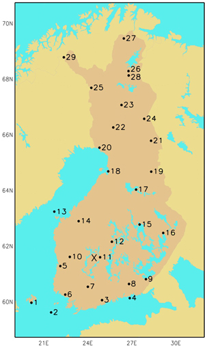
Fig. 1. Locations of the stations involved in this study. More information about the stations is presented in Table 1. The location of the Hyytiälä forestry field station is marked with a cross.
Precipitation measurements were discontinued during the early 2000s at many stations, particularly at most of the airport weather stations. At these locations, the measurement site for precipitation was accordingly changed, for some places even two or three times. This likely had little influence on the results because the compensatory stations are located close to the original measurement sites, and winter precipitation events causing heavy snow loads are mainly large-scale phenomena. Two stations included in the analyses, Suomussalmi and Salla, were completely closed down during the study period, and the time series of these stations were continued with the observations from new stations established close to the original ones. Additionally, discontinuities in the time series of Mariehamn and Lappeenranta were gap filled with observations from nearby stations. More detailed information about the changes in precipitation measurement sites and the replacement time series used for the other variables are presented in the footnote of Table 1. In addition, the time frames that were completely omitted from the analyses because of serious lack of data are likewise listed in Table 1.
| Table 1. Stations involved in this study along with their altitude above sea level and the geographical coordinates. The periods that have been excluded from the analyses because of missing data are listed as well. More information about the changes in measurement sites and data deficiencies are mentioned in the footnotes. | |||||
| No. | Station | Alt. (m) | Lat. (°N) | Lon. (°E) | Missing data |
| 1 | Mariehamn 1) | 5 | 60.12 | 19.90 | |
| 2 | Utö | 9 | 59.78 | 21.37 | |
| 3 | Vantaa | 51 | 60.33 | 24.96 | |
| 4 | Rankki 2) | 11 | 60.38 | 26.96 | Oct 2006 |
| 5 | Pori 3) | 13 | 61.47 | 21.79 | |
| 6 | Turku 4) | 49 | 60.52 | 22.27 | |
| 7 | Jokioinen | 104 | 60.81 | 23.50 | |
| 8 | Utti 5) | 99 | 60.89 | 26.94 | Dec 2010 |
| 9 | Lappeenranta 6) | 106 | 61.04 | 28.15 | Jul 2006 – Jun 2008 |
| 10 | Niinisalo | 124 | 61.84 | 22.46 | |
| 11 | Halli 7) | 145 | 61.86 | 24.79 | Jan 1961 – Dec 1964 |
| 12 | Jyväskylä | 139 | 62.40 | 25.68 | |
| 13 | Valsörarna | 4 | 63.44 | 21.06 | Jan 2009 – Dec 2010 |
| 14 | Kauhava 8) | 42 | 63.12 | 23.04 | |
| 15 | Kuopio 9) | 99 | 63.01 | 27.80 | |
| 16 | Joensuu 10) | 121 | 62.66 | 29.61 | |
| 17 | Kajaani 11) | 147 | 64.28 | 27.67 | |
| 18 | Oulu 12) | 14 | 64.93 | 25.35 | |
| 19 | Suomussalmi 13) | 220 | 64.90 | 29.01 | Jan 1961 – Aug 1970 |
| 20 | Kemi 14) | 19 | 65.78 | 24.58 | Jun 1995 – Nov 1999 |
| 21 | Kuusamo 15) | 264 | 66.00 | 29.22 | |
| 22 | Rovaniemi | 195 | 66.56 | 25.83 | |
| 23 | Sodankylä | 179 | 67.37 | 26.63 | |
| 24 | Salla 16) | 221 | 66.82 | 28.67 | |
| 25 | Alamuonio 17) | 252 | 67.97 | 23.67 | Nov 1982 – Jan 1983 |
| 26 | Ivalo 18) | 147 | 68.61 | 27.41 | |
| 27 | Kevo 19) | 107 | 69.76 | 27.01 | Jan 1961 – Dec 1961 |
| 28 | Kaunispää 20) | 430 | 68.43 | 27.44 | Jan 1961 – Oct 1995, Jul 2005 – Oct 2005, May 2008 – Oct 2008 |
| 29 | Kilpisjärvi 21) | 480 | 69.05 | 20.79 | Jan 1961 – Dec 1978 |
| 1) Measurement site for precipitation changed on 1st Oct 1995. All data is missing and replaced with data from a nearby station between 1st Oct 1995 and 3rd Sep 1999, 19th Dec 2003 and 5th Jan 2004, 31st Mar and 18th Jul 2005, 29th Dec 2008 and 7th Jan 2009, and 20th and 23rd Mar 2009. Most of these replacement time series have only four or three observations per day, depending on the variable. 2) Measurement site for precipitation changed on 1st Nov 2006. 3) Measurement site for precipitation changed on 1st Jan 2000 and 1st Jan 2010. 4) Measurement site for precipitation changed on 1st Jul 2006. 5) Measurement site for precipitation changed on 1st Jul 2009. 6) Measurement site for precipitation changed on 13th Jun 2008. All data is missing and replaced with data from a nearby station between 1st Oct 1995 and 27th Jun 1996. From 28th Jun 1996 until 29th Oct 1998 21 and 00 UTC observations are missing. 7) Measurement site for precipitation changed on 17th Jun 2009. 8) Measurement site for precipitation changed on 16th Nov 2009. 9) Measurement site for precipitation changed on 1st Jan 2005 and 1st Jan 2006. 10) Measurement site for precipitation changed on 1st Jan 2000. From 1st Jul 1996 until 28th Feb 1998 21 and 00 UTC observations are missing and from 1st Mar 1998 until 2nd Nov 1998 21, 00 and 03 UTC observations are missing. 11) Measurement site for precipitation changed on 1st Aug 2000. 12) Measurement site for precipitation changed on 1st Jun 2000, 1st Jul 2006 and 1st Jan 2008. 13) Measurement site for all variables changed on 1st Nov 2000. Relative humidity measurements are missing from 24th Oct 2005 until 1st Feb 2006. 14) Measurement site for precipitation changed on 1st Jun 1995 and 2nd Sep 2009. 15) Measurement site for precipitation changed on 30th Jun 2000. 16) Measurement site for all variables changed on 1st Aug 1999. Wind speed measurements are missing from 1st Jan 1968 until 19th Jan 1968. 17) Wind speed observations are available only four times per day between 1st Jan and 30th April 1961, and 1st Nov 1968 and 31st Jan 1969. 18) Measurement site for precipitation changed on 4th April 2000 and 1st Jan 2007. 19) All observations are available only three times per day in January 1962 and four times per day from 1st Feb 1962 until 31st Dec 1962. 20) Time series is extended to 30th Jun 2013. Precipitation is measured at a nearby station located at an altitude of 302 metres above the mean sea level. 21) Time series is extended to 30th Jun 2013. Until March 1998 most of 21 and 00 UTC observations are missing. | |||||
There is also some missing data in the periods included in the analyses. For example, many stations had missing data in April 1986 due to a civil servant strike, and short data breaks have become increasingly common after the 1990s because of automatised measurement systems. The missing data was treated as follows. Firstly, at some stations, observations were made only three, four, five, or six times per day during certain periods, which are mentioned in the footnote of Table 1. These periods were first gap filled. At the stations where six observations per day were conducted, 21 UTC and 00 UTC observations were missing, and they were replaced simply with the nearest observations made at 18 UTC and 03 UTC, respectively. When five observations per day were available, 03 UTC observations were missing in addition to 21 UTC and 00 UTC observations. In that case, the 21 UTC observations were replaced with the 18 UTC observations; the 03 UTC observations were replaced with the 06 UTC observations; and the 00 UTC observations were replaced with the average of 18 UTC and 06 UTC observations. Four observations per day were available when measurements were conducted every six hours and in that case, every second measurement missing compared to the three-hour observation interval was replaced with the average of the two nearest available observations. When only three observations per day were available the measurement times were 06 UTC, 12 UTC and 18 UTC. In that case, the missing 00 UTC observations were replaced with the average of 06 UTC and 18 UTC observations; the remaining missing values were gap filled similarly as in the case of the six-hour observation interval. During the second step of gap filling, all individual missing values were replaced with the average of the two nearest available observations, i.e., the observations made three hours before and three hours after the occasion of missing data. When at least two consecutive observations were missing, neither was replaced.
The amount of missing data after the gap filling and omitting of defective periods from the analyses varied among the stations and variables (Table 2). Clearly, most missing data existed at Kaunispää, where the proportion of missing data was 0.2% for precipitation and 2.6–4.0% for other variables. However, most of the missing data at Kaunispää occurred during summer. Precipitation time series generally had the fewest missing observations; for the other variables, the proportion of missing data was less than 0.5%, except for relative humidity at Suomussalmi and wind speed at Mariehamn. On average, wind speed observations showed the most missing data. In the cumulative crown snow-load calculations, the remaining missing data was treated so that the snow load was not allowed to increase while relevant weather information was missing, but the snow load was allowed to decrease, for instance, due to strong wind even without the temperature information and vice versa. To exemplify, snow load types not dependent on relative humidity were allowed to increase even while relative humidity data was missing and so on.
| Table 2. Proportions of missing data (‰) after gap filling at each station for temperature (T), relative humidity (RH), wind speed (U) and precipitation (P) within the periods included in the analyses. | |||||
| No. | Station | T (‰) | RH (‰) | U (‰) | P (‰) |
| 1 | Mariehamn | 2.9 | 4.2 | 14.0 | 0.0 |
| 2 | Utö | 0.2 | 0.7 | 2.2 | 0.0 |
| 3 | Vantaa | 1.6 | 1.7 | 1.7 | 0.0 |
| 4 | Rankki | 0.0 | 0.0 | 4.8 | 0.0 |
| 5 | Pori | 0.9 | 2.1 | 2.0 | 0.0 |
| 6 | Turku | 0.5 | 0.6 | 0.7 | 0.0 |
| 7 | Jokioinen | 0.0 | 0.1 | 0.6 | 0.0 |
| 8 | Utti | 0.1 | 0.2 | 1.1 | 0.1 |
| 9 | Lappeenranta | 0.7 | 2.4 | 2.4 | 0.0 |
| 10 | Niinisalo | 0.0 | 0.0 | 0.0 | 0.0 |
| 11 | Halli | 0.5 | 1.1 | 0.8 | 0.0 |
| 12 | Jyväskylä | 0.1 | 0.6 | 0.5 | 0.0 |
| 13 | Valsörarna | 0.0 | 1.3 | 2.1 | 0.0 |
| 14 | Kauhava | 0.5 | 0.7 | 1.4 | 0.0 |
| 15 | Kuopio | 0.2 | 1.0 | 1.0 | 0.0 |
| 16 | Joensuu | 0.1 | 1.7 | 1.7 | 0.0 |
| 17 | Kajaani | 0.1 | 1.1 | 1.7 | 0.0 |
| 18 | Oulu | 0.6 | 1.6 | 1.8 | 0.2 |
| 19 | Suomussalmi | 0.2 | 7.4 | 0.8 | 0.0 |
| 20 | Kemi | 2.2 | 3.4 | 3.5 | 0.0 |
| 21 | Kuusamo | 0.3 | 1.3 | 1.6 | 0.0 |
| 22 | Rovaniemi | 0.0 | 0.3 | 0.3 | 0.0 |
| 23 | Sodankylä | 0.0 | 0.9 | 0.8 | 0.0 |
| 24 | Salla | 0.0 | 0.0 | 1.1 | 0.0 |
| 25 | Alamuonio | 0.0 | 3.8 | 3.3 | 0.0 |
| 26 | Ivalo | 0.6 | 1.7 | 1.8 | 0.0 |
| 27 | Kevo | 0.3 | 0.3 | 0.8 | 0.0 |
| 28 | Kaunispää | 37.6 | 25.9 | 40.1 | 2.4 |
| 29 | Kilpisjärvi | 0.0 | 2.2 | 3.1 | 0.0 |
For our purposes, the quality of observations was substantially worse for wind speed than for other variables. That is because the wind speed observations are not necessarily comparable between different stations or times. Wind speed is usually measured routinely at 10 metres in an open location. At some stations, the wind speed measurements are conducted over forest, and in that case, the measurement height is typically approximately ten metres above the forest canopy. Measurement heights and locations have also changed at some stations even several times during the study period, and some of the earliest changes were not documented. In addition, wind conditions have slowly changed at many measurement sites because of forest growth and changes in other factors affecting the local wind climate. Therefore, we decided not to apply any correction to wind measurements, as it would be impossible to produce truly homogenous wind statistics. At least in one case, wind speeds were systematically reduced simultaneously with a documented increase in measurement height. Thus, correcting the observations by, for example, assuming the logarithmic wind profile, would have led only to an increase in the error.
Some inhomogeneity exists also in the time series of other variables in addition to wind speed. For instance, precipitation observations are known to be sensitive to wind-induced undercatch, particularly in the case of solid precipitation (Yang et al. 1999; Sugiura et al. 2006). In order to reduce this undercatch, wind shields of all FMI rain gauges were changed in the 1980s from Wild to Tretyakov. These restrictions in data quality have to be kept in mind when interpreting the results of this study.
2.2 REFI-B data
In addition to the above-described data set, we used an observational 30-year data set prepared in the context of the Climatological Test Years in Finland for Building Physics (REFI-B) research program (Ruosteenoja et al. 2013). The REFI-B data set consists of years 1980–2009 and includes meteorological observations interpolated to an hourly interval at four locations: Vantaa, Jokioinen, Jyväskylä and Sodankylä. The REFI-B data originates essentially from the same data that is described above, but it additionally includes global radiation, and daily precipitation sums are divided very approximately to an hourly interval based on surface synoptic observations made every three hours.
2.3 Data from the Hyytiälä research station
In assessing the model performance, we used daily digital images of canopy snow cover from the Hyytiälä forestry field station. The location of Hyytiälä in Finland is shown in Fig. 1. The images encompass three consecutive winter seasons (2008/09–2010/11) and were classified visually into six classes. The classification criteria of canopy snow are originally presented by Kuusinen et al. (2012). The canopy snow classes are as follows: 0= canopies are snow free; 1 = most of the canopy is snow free; 2 = nearly equal amounts of snow-covered and snow-free surfaces are visible in the canopy; 3 = most of the branches and needles are covered with snow, but some are bare; 4 = no snow-free branches or needles are visible in the canopy; and 5 = canopies are snow free but covered with rime or hoarfrost. As discussed by Kuusinen et al. (2012), the classification is subjective and thus approximate, not exact.
To model the crown snow loads at Hyytiälä, we used temperature, wind speed, global radiation and precipitation observations from the Station for measuring ecosystem–atmosphere relations (SMEAR II) (Hari and Kulmala 2005) averaged over 30-minute time steps and achieved through the SmartSearch online tool (Junninen et al. 2009). For relative humidity, we used observations from the weather station of FMI at Hyytiälä because the relative humidity measurements at SMEAR II proved to be flawed. At SMEAR II, wind speed is measured in a measurement tower situated in a pine forest approximately 15 metres high. Because in the crown snow-load calculations wind speed is intended to be measured at 10-metre height in an open place, we estimated wind speed at 10 metres above the forest canopy (i.e., a 25-metre height) on the basis of measurements conducted at 16.8- and 33.6-metre heights by applying the logarithmic wind profile under neutral conditions (Holton 2004):

where U is wind speed (m s–1) at height z (m), u* is the friction velocity (m s–1), κ is the von Kármán’s constant (≈0.4) and zo is the roughness parameter (m). On average, the estimated wind speed at 25-metre height proved to correspond closely the observed 10 metres wind speeds at the nearest airport weather stations at Halli and Jyväskylä.
2.4 North Atlantic Oscillation
In the results section, we compare the modelled occurrence of different snow-load types with North Atlantic Oscillation (NAO) index values. The NAO indices were obtained from the Climate Prediction Center at the National Centers for Environmental Prediction (http://www.cpc.ncep.noaa.gov/). The NAO basically describes fluctuations in the difference of atmospheric pressure at sea level between Iceland and the Azores. It has been frequently used to illustrate the effect of large-scale circulation anomalies on winter weather in Europe. In Northern Europe, strong positive (negative) phases of NAO tend to be associated with above (below) normal temperatures in winter. The connection between NAO and winter weather is discussed in more detail by Visbeck et al. (2001).
3 Methods
3.1 Crown snow-load calculations
We estimate the amount of crown snow loads based on the FMI model and the G08 method. The FMI model is based on the experimental work and knowledge of several experts. The model has been used operationally at FMI to predict heavy crown snow loads since 2006, and during this time, the parameters of the model have been tuned based on the experience of model performance in different weather situations. The model parameters are thus empirical and based on statistics, not physics. The model is still by no means perfect, and definitive improvement of the model would require a thorough measurement campaign of actual crown snow loads in different environments and weather situations.
The FMI model assumes an exemplar tree that has a cone-shaped crown with a projected catchment area of one square metre from above and from the side in the direction of the wind. For example, a cone-shaped spruce crown with a height of 1.77 m and a bottom circle radius of 0.56 m fulfils that assumption. It is further assumed that a 1-mm water layer of melted snow load on a horizontal surface corresponds to a 1-kg m–2 snow load on the tree crown.
The FMI model uses a time step of one hour, and the model works as follows. First, part of the existing snow load is transformed into a different type according to weather conditions if needed. The snow load is classified into four types in the model: rime, dry snow, wet snow, and frozen snow. After that, the snow load is increased and decreased because of snow accretion and removal. Decrease of the snow load in the model is due to dropping and melting induced by wind and thaw. In addition, high solar radiation decreases the load because solar radiation can warm up the branches and needles of trees above the freezing point and induce dropping of snow even with cold air temperatures. Increasing the snow load is caused by accumulation of rime and snowfall. Finally, the calculations are repeated for the next time step. Appendix A in the supplementary material contains a detailed description of the calculation procedure, including equations. Weather variables needed in the calculations are air temperature and relative humidity measured at 2-metre height, 10-minute average wind speed measured at 10 metres, precipitation, global radiation, and cloudiness. In addition, the elevation of terrain above sea level affects the riming efficiency in the model. In this study, the effect of cloudiness is omitted. Cloudiness affects only the calculation of rime accretion, and this is thus assumed to have little effect on the results because the weather situations favourable for riming (high relative humidity, moderate or high wind speed and air temperature mostly between 0and –5 °C) are in any case cloudy by a large majority. Moreover, solar radiation has only a limited effect on the modelled crown snow loads as it decreases the snow loads virtually only in late winter and spring as discussed in the next section. Hence, and because global radiation time series are available only from a few stations, we also omitted the effect of solar radiation in most of the calculations. We note that in reality, cloudiness controls the outgoing radiation and can thus also affect freezing of wet snow.
In calculating the crown snow loads based on the data described in Section 2.1, the values of weather variables observed every three hours were linearly interpolated to an hourly interval during the calculation procedure. The daily precipitation sums were uniformly distributed for each 24-hour period. The effect of this smoothing of precipitation on the results is discussed in Section 4. The interpolation method used for temperature, relative humidity and wind speed observations is the same that was applied in the preparation of the REFI-B data set.
The G08 method to calculate the crown snow loads presented by Gregow et al. (2008) is simpler. It has a 3-hour time step and uses as input variables 2-metre air temperature, average wind speed measured at 10-metre height and precipitation. In this model, the snow load is changed by loss of snow due to wind removal and melting and by accumulation of snowfall, sleet and even rain when the temperature is below 2.3 °C. The expression for the loss of snow load (%) by melting is as follows:
where T is the 2-metre air temperature (°C). The snow removal by wind (%) is calculated as follows:
![]()
where U is the 10-minute average wind speed (m s–1) at 10-metre height. The snow load (kg m–2) is calculated for every time step n based on Eqs. 2 and 3 and the amount of precipitation (P) in liquid water (mm) as follows:
In Eq. (4) are included every form of precipitation which can vary between wet snow, graupel, sleet, drizzle and rain in temperatures slightly above the freezing point. That is because the wetter the snow becomes, the heavier the load gets and even rain can thus increase the weight of the snow load.
3.2 Number of risk days for heavy riming and snow loading
In addition to the modelled crown snow-load amounts, we defined the numbers of potential days for heavy rime and total snow load accretion across Finland on the basis of observed daily mean values of air temperature, relative humidity, wind speed and precipitation. The aim was to find out how closely the geographical distribution of risk days favourable for heavy rime and snow accretion determined based on the daily means of the above-mentioned weather variables corresponds with the modelled heavy rime and total crown snow-load amounts.
To derive the connection between the number of risk days and daily means of weather variables, we used the REFI-B data and the FMI model. First, we determined the limits on daily increases of modelled total crown snow and rime loads occurring on average twice a year. The daily increases were calculated by comparing the modelled maximum loads on two consecutive days. Within the period 1980–2009, this limit for the total snow load varied in Jokioinen, Jyväskylä, Sodankylä and Vantaa between 5.0 and 6.1 kg m–2 and for the rime load between 1.4 and 2.0 kg m–2, depending on the location. The average values were 5.35 kg m–2 for the total crown snow load and 1.72 kg m–2 for the rime load. Next, these average values were used to search for typical weather conditions prevailing in days with heavy snow loading or riming. For each of the four stations, we determined the range of daily mean values for air temperature, relative humidity, wind speed and precipitation, separately for each variable, on which 90% of days with increases in the load exceeding the limit value (i.e., 5.35 or 1.72 kg m–2) fell within. Finally, all the days when the daily means for all of those variables fell within the 90% interval were considered as risk days. The final threshold values shown in Table 3 for daily mean temperature, relative humidity, wind speed and precipitation to determine the risk days were defined as an average of those for Jokioinen, Jyväskylä, Sodankylä and Vantaa.
| Table 3. Threshold values of daily mean 2-metre air temperature (Tmean), 2-metre relative humidity (RHmean), 10-metre wind speed (Umean) and total precipitation (Pday) that are used to determine the risk days favourable for heavy snow loading and riming. | |
| Snow-loading | Riming |
| –3.42 °C < Tmean < 1.05 °C | –5.19 °C < Tmean < –0.16 °C |
| RHmean > 89.44% | RHmean > 95.50% |
| 2.07 m s–1 < Umean < 5.63m s–1 | 2.00 m s–1 < Umean < 4.54 m s–1 |
| Pday > 6.41 mm | Pday < 1.11 mm |
Not on every risk day do the crown snow loads actually increase substantially. At each location, during less than half of the risk days for heavy snow loading, the total crown snow load increase exceeded 5.35 kg m–2, but during most of the risk days for heavy riming, the increase in rime load indeed surpassed 1.72 kg m–2. On the other hand, heavy snow loads occur occasionally also on days that do not meet the above-described criteria for a risk day. Hence, these thresholds values should not be used to detect exact heavy snow-load events, but the criteria are rather suited to locate the geographical areas with the highest risk. It should also be noted that the events of which frequency the numbers of risk days are intended to describe are fairly common, occurring approximately twice a year, whereas the crown snow loads heavy enough to cause actual forest damage are much more rare and coincidental. According to Solantie (1994), the snow loads sufficient to break individual large tree stems occur in Finland every 3 to 17 years depending on the location. For example, in the region of Uusimaa, which is recognised as one of the most susceptible regions for snow damage in southern Finland, severe snow damage has occurred in recent decades during the winters 1958/59, 1984/85 and 1991/92 (Solantie 1994).
3.3 Kriging interpolation
To create nationwide spatial analyses of the parameters describing the crown snow-load conditions in Finland, we applied the kriging interpolation method (Goovaerts 1997). Kriging is a widely used method for creating gridded spatial analyses of meteorological and climatological variables from point values. It has been applied both in regional (e.g., Vajda and Venäläinen 2003) and nationwide studies (e.g., Aalto et al. 2013) as well as in creating continental-scale gridded analyses (Hofstra et al. 2008). In kriging, point values are interpolated into areas between observation stations based on the observational data and the spatial autocorrelation of the observations, as well as on the environmental factors affecting the parameter in question. In this study, we applied kriging with external drift (Aalto et al. 2013), and the environmental factors taken into account in the interpolation were the mean elevation above sea level and the percentages of lake and sea cover in a grid square. The interpolation was performed on a 10 km x 10 km grid covering Finland. The accuracy of the interpolation is affected by the density of the observation network and the terrain complexity. Because we performed the interpolation based on only 29 stations, small-scale spatial features could not be described in great detail. Particularly in Lapland, where altitude variations are greater than elsewhere, the interpolation is inaccurate.
4 Model performance
4.1 Model evaluation against the canopy snow classification
In this section, we evaluate the capability of the FMI model to reproduce realistic crown snow loads. The model performance is further compared with the G08 method. The daily course of the simulated crown snow loads by both methods at Hyytiälä during the three consecutive winters 2008/09–2010/11 is presented in Fig. 2, with the canopy snow classification simultaneously. In Fig. 3, we illustrate the variability of the modelled snow loads among individual canopy snow classes. Here, we also present the statistics for the modelled snow loads when daily averages of all the needed weather variables have been used in the calculations as input instead of hourly values, because the G08 method has been previously implemented in climate change studies applying the daily mean values (Gregow et al. 2011).
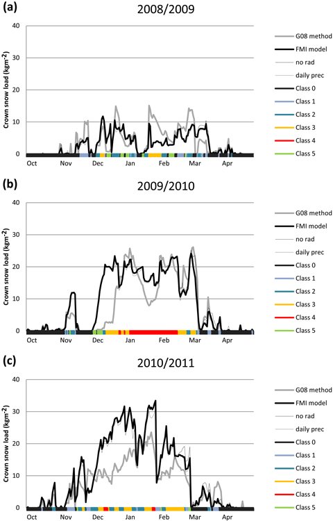
Fig. 2. The daily total crown snow loads (kg m–2) at Hyytiälä on 12 UTC calculated by the G08 method (thick grey line) and the FMI model (thick black line) during the winter (a) 2008/2009, (b) 2009/2010 and (c) 2010/2011. The crown snow loads calculated by the FMI model but excluding the effect of solar radiation (thin solid line) and by using daily precipitation sums instead of hourly sums in the calculations (thin dashed line) are shown as well. The classification of days into six canopy snow classes is presented with colour bars along the x-axis.
Fig. 2 shows that during the 2008/09 winter, both the modelled and visually estimated crown snow loads were on average clearly smaller than during the next two winters. The winters of 2009/10 and 2010/11 were, in general, both characterised with cold and snowy weather in Finland. Abundant crown snow loads were observed during both of these winters but particularly from late December 2009 until mid-February 2010, the crown snow loads remained very large. This is a particularly interesting period for the model verification, since this episode has been documented to cause forest damage in the area (Vastaranta et al. 2012). Based on the FMI model, the crown snow loads varied at around 20 kg m–2 throughout the episode. The maximum loads exceeded 20 kg m–2 also on the basis of G08 method, but the load decreased below 10 kg m–2 in mid-January based on that method, although in reality, the snow loads remained stable. Temperature varied at Hyytiälä in January 2010 mostly between –5 and –30 °C, winds were mainly weak and virtually any notable precipitation did not occur for weeks. Under these conditions, the FMI model seemed to maintain the snow load better because even weak winds gradually reduced the snow load calculated by the G08 method, whereas in the FMI model, wind speed has to exceed a certain threshold in order to reduce the load.
Another specifically interesting period was the first fortnight of December 2009. During this period, very favourable conditions for riming prevailed for several days but the tree canopies were at the same time almost entirely free from fallen snow. As the G08 method does not take riming into account, the crown snow loads were low based on that method. Notwithstanding, the FMI model suggested the snow load increase simultaneously up to 20 kg m–2 almost exclusively due to rime accretion. Though during the second week of December, the tree branches were clearly bent down due to heavy rime loads, the total crown snow loads were admittedly clearly lower than later in January when the modelled loads were still close to 20 kg m–2. Thus, the FMI model most likely somewhat overestimated the rime accretion. This is, furthermore, the general feeling among the duty forecasters at FMI that the model usually slightly overestimates the rime accretion. It can also be noted that the exclusion of the effects of cloudiness in the calculations did not affect the results in this case because overcast conditions prevailed throughout the riming period.
During the third winter of 2010/11, the modelled crown snow loads at Hyytiälä were mostly even larger than during the 2009/10 winter, especially on the basis of the FMI model. Both the winters of 2009/10 and 2010/11 were, furthermore, slightly unusual in that regard considering that the majority of the total crown snow load simulated by the FMI model consisted of rime. The modelled crown snow-load amounts were more or less realistic as snow loads of ~20–30 kg m–2 are known to be able to cause uprooting in pine forests and stem breakages in unmanaged stands (Päätalo 2000). Furthermore, it is likely that riming played a critical role in causing the snow damage because the damage that occurred at Hyytiälä in 2010 were restricted to the areas with an elevation of at least 160 metres above sea level (Vastaranta et al. 2012).
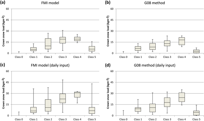
Fig. 3. Box plots showing the distribution of calculated crown snow loads among the different canopy snow classes at Hyytiälä during the period from April 1, 2008 to April 30, 2011. The boxes indicate the central 50% range and the median of the distribution of calculated crown snow loads on days falling into a canopy snow class in question. The whiskers extend to the fifth and 95th percentiles of the distribution. The results are presented for (a) the FMI model and (b) the G08 method. We also show the statistics for the snow loads when daily mean values of all needed input variables are used in the calculations for (c) the FMI model and (d) the G08 method.
Based on Fig. 3, it is not obvious whether the FMI model or the G08 method performs better in simulating the crown snow-load amounts. The simulated loads by both methods increase, on average, with increasing canopy snow amounts. This feature is still visible when daily averages are used as input, although variability among individual snow classes greatly increases in that case. The snow loads simulated by the FMI model are, on average, slightly larger than those based on the G08 method. This is partly because two of the three winters used in the verification exhibited relatively heavy rime loads. On the other hand, located at a rather high altitude when compared to the surrounding areas, the rime loads at Hyytiälä are also, in general, relatively large. The clearest difference between the two methods occurs on days classified into Class 5 when the canopies are snow free but covered with rime. In that case, heavier loads were, on average, simulated with the FMI model than by the G08 method because the latter does not take riming into account. On days classified into Snow Classes 2 and 3, the variability among the simulated snow loads was higher for the FMI model than for the G08 method and vice versa on the days classified into Class 4. However, a large majority of the days classified into Class 4 was due to a single episode and hence, the result may not be generalised. The lower tail of distribution of simulated crown snow loads on the days classified into Class 4 is shorter for the FMI model than for the G08 method because the G08 method slowly decreased the snow loads in January 2010.
Furthermore, we can see from Fig. 2 that omitting the effects of solar radiation in the calculations only has an effect in late winter and spring. On average, the simulated afternoon crown snow loads at Hyytiälä were 2%, 25% and 7% larger in February, March and April, respectively, when the effect of solar radiation was omitted in the FMI model. Thus, we think that omitting the effect of solar radiation does not have a significant effect on the results when the spatial occurrence of heavy crown snow loads over Finland is studied. Another aspect that can be seen from Fig. 2 is that the results are even surprisingly similar, irrespective of whether hourly or daily precipitation sums are used in the calculations. Approximately 5% of lower snow loads were simulated on average when daily precipitation sums were used instead of hourly ones. Of course, the effect can be much greater on individual cases, but also in the REFI-B data set, the correlation between the crown snow loads calculated with daily and hourly precipitation sums proved to be 0.99, although the hourly sums in that data set are already smoothed. When daily mean values of all the weather variables needed as input data in the FMI model were used, the correlation between the snow loads calculated based on the hourly values was, on average, 0.82 in the REFI-B data. This proved to still be a somewhat higher value than the correlation between the snow load amounts calculated with the FMI model and the G08 method. The use of daily mean values as input gave better estimates for rime and dry snow loads than for wet snow and frozen snow loads.
4.2 Case studies
Here, we briefly exemplify the performance of the FMI model in operational use with the help of two real cases when snow damage had occurred. In the operational use, the model is run both based on the forecasted and observed weather data. The observation-based analysis is performed applying an operational mesoscale analysis system called Mesan (Häggmark et al. 2000). The Mesan produces a gridded analysis of several weather parameters combining information from all available different kinds of observations that include manual and automatic station observations, as well as satellite and weather radar imagery. This observational analysis of the modelled crown snow loads then provides initial conditions for snow-load forecasts. The forecasted snow loads are further calculated based on the output of a numerical weather prediction (NWP) model that has been edited first by a duty forecaster. The NWP models that are frequently used at FMI are the High Resolution Limited Area Model (Undén et al. 2002) and the Integrated Forecast System of the European Centre for Medium-Range Weather Forecasts (ECMWF 2014).
The first exemplified case occurred in the turn of October and November 2008 when heavy wet snow leaned and bent trees over power lines causing a lot of blackouts in the region of Kainuu. Based on the forecast, crown snow loads should have surpassed 20 kg m–2 on the evening of October 31 locally in Kainuu (Fig. 4). Authorities were, for the first time, informed about the risk of snow damage on the previous day and the forecast was amended on October 31. Altogether, about 3000 customers suffered power cuts in Kainuu (Fig. 4e) within this episode between October 31 and November 2. During this episode, precipitation widely exceeded 20 mm and at the most approximately, 35 cm of wet snow had fallen on the ground. Within the areas that suffered most, the temperature was mostly between 0and 0.5 °C during the snowfall enabling the effective lodging of wet snow on trees.
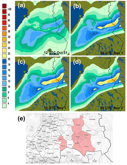
Fig. 4. Total crown snow loads (kg m–2) forecasted by the FMI model for (a) 12 UTC on October 31; (b) 00 UTC on November 1; (c) 12 UTC on November 1; and (d) 00 UTC on November 2 in 2008. The snow loads exceeding 20 kg m–2 are shown with yellowish colours. (e) The municipalities where snow damages caused power cuts are shown in light red.
The second example is from January 2012. During this case, forest damage caused by heavy crown snow loads that were both because of wet snow and rime accretion inflicted interruptions in the electricity supply at many locations in southern and central Finland. In the central parts of the country, the situation was made worse because crown snow loads were already relatively high before the event. On the basis of the FMI model forecasts, authorities were warned about the case on January 10. On January 12 and January 13, emergency centres received numerous notifications concerning snow damage from the regions of Satakunta, Pirkanmaa, Päijät-Häme and Kymenlaakso in southern and south-western Finland. Observational analysis of the situation reveals that the FMI model was able to locate these areas with the greatest risk well (Fig. 5).
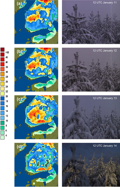
Fig. 5. Total observational crown snow loads (kg m–2) simulated by the FMI model for (a) 12 UTC on January 11; (b) 12 UTC on January 12; (c) 12 UTC on January 13; and (d) 12 UTC on January 14 in 2012. The snow loads exceeding 20 kg m–2 are shown with yellowish colours. Images of canopy snow at Hyytiälä on the corresponding moments are presented as well. The location of Hyytiälä is shown on the maps with a black dot.
5 Spatial and temporal occurrence of heavy crown snow loads
Based both on the FMI model and the G08 method, the crown snow loads achieved in Finland once a year are, on average, greatest along the Russian border (Fig. 6), whereas, the smallest crown snow loads are experienced in the coastal areas of southern and western Finland. The maximum loads based on the FMI model are consistently somewhat larger than those on the basis of the G08 method, although the situation is locally opposite in north-western Lapland. It is furthermore visible that the area of heaviest snow loads is concentrated more or less farther north based on the G08 method than based on the FMI model.
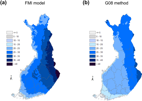
Fig. 6. The spatial distribution of the crown snow-load amount (kg m–2) achieved on average on one day per year within the period 1961–2010 on the basis of (a) the FMI model and (b) the G08 method.
The spatial distribution of different crown snow-load types (Fig. 7) resembles the distribution of heavy total snow loads. For every snow load type, the heaviest loads seem to occur in eastern Finland on average. Nevertheless, some differences are visible in the spatial patterns of different snow-load types. For instance, the heaviest wet snow loads are concentrated farther south than the heaviest dry snow loads. In addition, it can be noted that the dry snow loads obtained on average once a year are clearly lower than the loads of other snow types occurring with an equal frequency over most of the country. Consequently, dry snow is obviously the least important snow type with regard to snow damage. However, when compared to Fig. 6b, we see that among the different snow types, the spatial pattern of dry snow resembles most closely that of heavy crown snow loads modelled by the G08 method. Lastly, we note that the spatial distribution of heavy rime loads seems to have more small-scale features than the distributions of other snow types. This is admittedly because riming is strongly affected by the local topography.
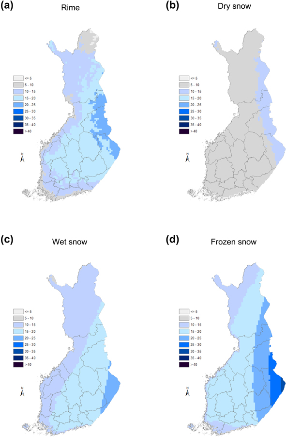
Fig. 7. The spatial distribution of (a) rime; (b) dry snow; (c) wet snow; and (d) frozen snow-load amount (kg m–2) achieved on average on one day per year within the period 1961–2010 on the basis of the FMI model.
The numbers for risk days for heavy rime and total snow-load accretion are displayed in Fig. 8. For the accretion of the total snow load, the spatial pattern of risk days resembles noteworthily the geographical distribution of heavy wet snow loads (Fig. 7e). Among the stations involved in this study, correlation between these two variables proved to be 0.81 while it is only 0.68 between the total crown snow loads occurring on one day per year, on average, and the number of risk days for heavy total crown snow-load accretion. Thus, the number of risk days for heavy total snow load accretion best describes the specific risk for snow damage caused by wet snow. This is understandable because the wet snow hazards are typically swift events that can escalate even during the same day when the accumulation of snow begins. The spatial pattern of the number of risk days for heavy rime accretion does not follow as closely the spatial pattern of heavy rime loads (Fig. 7a). Most risk days are found in the inland regions of south-western Finland (Central Finland, Pirkanmaa, Kanta-Häme and Päijät-Häme), whereas the heaviest rime loads were modelled to occur in north-eastern parts of the country (regions of North Karelia, Kainuu and Koillismaa). This discrepancy is possibly related to the fact that heavy rime loads usually develop over relatively long periods of time and thaw periods that dislodge the load are more common in the southern and western parts of the country.
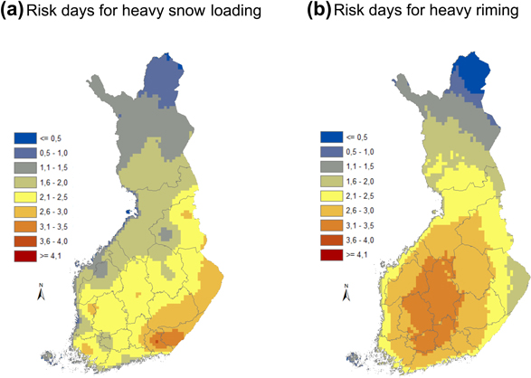
Fig. 8. The annual average count of risk days for (a) heavy snow loading and (b) heavy riming within the period from 1961–2010.
In Fig. 9, we further illustrate the connection between the number of risk days and the days when snow load has actually increased. The number of risk days for heavy total snow load accretion has a strong positive correlation with the number of days when the modelled total snow loads have actually increased substantially. Between the number of risk days for heavy rime accretion and the number of days with modelled increase in the rime loads, there is more scatter. A more detailed inspection reveals that at most of the locations, the numbers for risk days and accretion days for the rime loads correspond closely but at the maritime locations, and especially at those stations in northern Finland that are located at high elevations, the numbers for risk days are notably underestimated. The number of days when strong rime accretion was modelled is clearly highest at Rovaniemi and Kaunispää, two stations in northern Finland located at a high elevation as compared to the surrounding areas. Because maritime stations (Rankki, Utö and Valsörarna) also exhibited too few risk days for heavy riming, it can be concluded that the threshold values determined for the risk days for heavy riming in this study are not very suitable at windy locations. More specifically, the modelled rime accretion at Kaunispää was at its own level as compared to other locations: the greatest modelled daily increase in the rime load was there even 9.0 kg m–2 while 1.72 kg m–2 was used as a threshold value for the heavy daily rime load increase. This is why Kaunispää is the one station that also sticks out in Fig. 9a because riming solely increases occasionally even the total crown snow loads there enough to surpass the daily threshold used to detect the days with heavy snow loading. However, on average the modelled rime loads were not largest at Kaunispää because high winds frequently dislodge the load in the model.
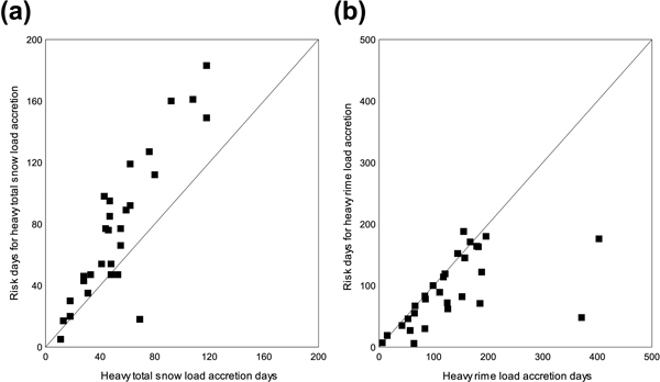
Fig. 9. Number of risk days for (a) heavy total snow-load accretion as a function of the number of days with modelled heavy total snow load accretion; and (b) heavy rime load accretion as a function of the number of days with modelled heavy rime accretion.
The occurrence of heavy snow-loading events in Finland has discernible seasonality. Riming events concentrate strongly on late autumn and early winter, but the number of days when the total crown snow load increases substantially has a bimodal seasonal distribution peaking both in early and late winter (Fig. 10). This is because these events are usually associated with wet snow accretion that can only occur when the temperature is close to 0°C. The early winter peak is still much greater than the one in late winter. In northern Finland, heavy snow loads occurs most in October, in central Finland in November and in southern Finland from November to January. Heavy riming occurs rather similarly in the north most already in October and in the south from November to January. In the north, a few heavy riming events occur even during late winter and spring but almost exclusively only at Kaunispää, which is located on a fell top.
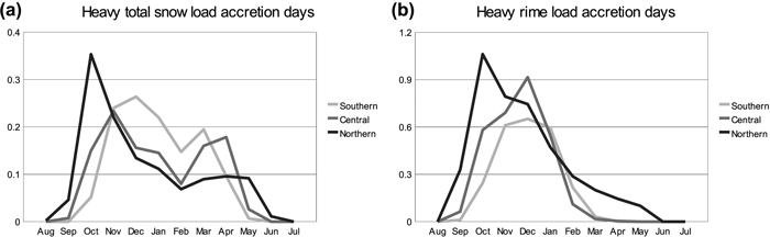
Fig. 10. Annual average number of days by month when (a) the modelled daily maximum total snow load has increased at least 5.35 kg m–2 as compared to the maximum of the previous day; and (b) the modelled daily maximum rime load has increased at least 1.72 kg m–2 as compared to the maximum of the previous day. Statistics are shown separately for southern (stations 1–9), central (stations 10–19) and northern (stations 20–29) Finland.
In Table 4, we present the correlation coefficients between the annual wintertime (November–March) mean weather variables and the occurrence of different snow load types. Wind speed is found to correlate negatively with the occurrence of all kind of snow load types throughout the country and, contrary to that, relative humidity seems to correlate positively with the occurrence of every snow-load type. Most significant these correlations are between relative humidity and rime loads and between wind speed and dry snow loads. This is unsurprising, as riming efficiency in the model is directly proportional to wind speed and dry snow is most easily blown away by wind. The amount of precipitation has the strongest positive correlation with the wet snow loads. Particularly in central and northern Finland, temperature also correlates positively with the wet snow loads. The rime and frozen snow loads correlate differently with temperature between the southern and northern parts of the country. In the south, heavier loads occur during cold winters and in the north during mild winters. Furthermore, we present the correlation coefficients between the wintertime NAO index values and the occurrence of the snow-load types. These correlations are relatively weak and they more or less follow the correlations between temperature and the occurrence of the snow-load types. This is because NAO is positively correlated with winter temperatures in Finland. To conclude, in southern Finland, somewhat heavier crown snow loads seem to typically occur during relatively cold winters than during mild winters and vice versa in the north.
| Table 4. Correlation coefficients between the annual November–March mean temperature (T), relative humidity (RH), wind speed (U), precipitation (P) and NAO index values and the modelled annual number of days with rime (Nrime), dry snow (Ndry snow), wet snow (Nwet snow) and frozen snow (Nfrozen snow) loads exceeding the value achieved on average on ten days a year. The correlations are shown as an average of the stations in southern (stations 1–9), central (stations 10–19) and northern (stations 20–27) Finland as well as an average of all stations excluding the short time series of the stations 28 and 29. On individual stations, correlations above 0.3 and below –0.3 are statistically significant. | ||||
| Southern | Central | Northern | National | |
| T & Nrime | –0.3 | –0.1 | 0.1 | –0.1 |
| T & Ndry snow | –0.3 | –0.1 | –0.1 | –0.1 |
| T & Nwet snow | 0.1 | 0.4 | 0.3 | 0.3 |
| T & Nfrozen snow | –0.1 | 0.1 | 0.3 | 0.1 |
| RH & Nrime | 0.4 | 0.5 | 0.5 | 0.5 |
| RH & Ndry snow | 0.2 | 0.2 | 0.1 | 0.2 |
| RH & Nwet snow | 0.3 | 0.2 | 0.1 | 0.2 |
| RH & Nfrozen snow | 0.2 | 0.1 | 0.1 | 0.2 |
| U & Nrime | –0.4 | –0.3 | –0.1 | –0.3 |
| U & Ndry snow | –0.6 | –0.5 | –0.5 | –0.5 |
| U & Nwet snow | –0.2 | –0.1 | –0.2 | –0.2 |
| U & Nfrozen snow | –0.3 | –0.3 | –0.2 | –0.3 |
| P & Nrime | –0.2 | 0.0 | 0.1 | –0.1 |
| P & Ndry snow | 0.1 | 0.2 | 0.3 | 0.2 |
| P & Nwet snow | 0.3 | 0.5 | 0.5 | 0.4 |
| P & Nfrozen snow | 0.1 | 0.2 | 0.3 | 0.2 |
| NAO & Nrime | –0.3 | –0.1 | 0.0 | –0.2 |
| NAO & Ndry snow | –0.2 | 0.0 | 0.1 | 0.0 |
| NAO & Nwet snow | 0.2 | 0.3 | 0.2 | 0.2 |
| NAO & Nfrozen snow | 0.0 | 0.1 | 0.1 | 0.1 |
Lastly, we explore possible trends in the crown snow-load amounts over the period 1961–2010. Because most of the observational time series were corrupted due to inhomogenities in wind measurements and the crown snow loads are, on average, negatively correlated with wind speed, we confine this exploration only to those stations where no significant trend in November–March average wind speed could be detected. In addition, Kaunispää and Kilpisjärvi were ruled out because of their short time series. This only restricts the inspection to eight stations, which are Vantaa, Turku, Utti, Niinisalo, Halli, Kauhava, Salla and Kevo. The time series for several variables describing the heavy crown snow loads are presented in Fig. 11. All of the time series that are shown exhibit a slight increasing trend, but the trend is not statistically significant for any variable. In individual locations, some of the trends nevertheless proved to be significant. Statistically significant increasing trends were detectable in 0–3 locations out of eight, depending on the variable. Decreasing trends were apparent only at Vantaa and for the total snow loads. However, among the eight stations included in this analysis, wind measurements were most questionable at Vantaa as the increasing trend in wind speed there just failed to be statistically significant. It is likely the case that the expansion of the airport area in the 1990s has affected the local wind climate there. Moreover, the heaviest snow loads simulated at Vantaa occurred in December 1961 during the very first winter of the time series.
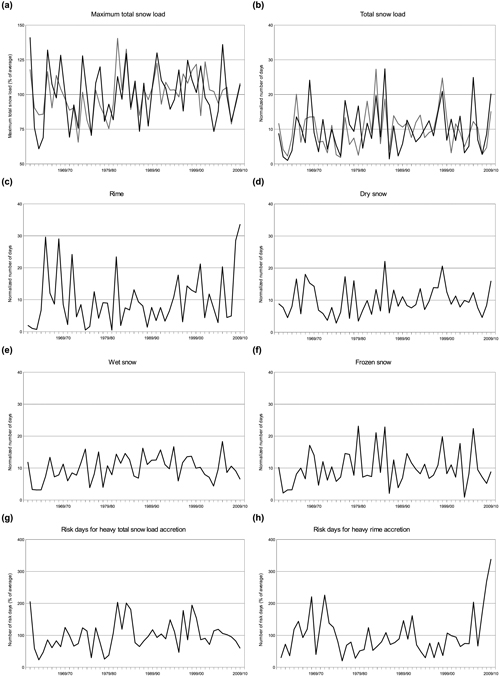
Fig. 11. Temporal variation of modelled heavy snow loads in Finland within the winters between 1961/62–2009/10 as an average of those eight stations where no significant trend in November–March wind speed was apparent during the same period. Variables that are presented are as follows: (a) the maximum annual crown-snow load (% of average) based on the FMI model (black line) and the G08 method (grey line); (b) the annual number of days with the total crown snow load exceeded the value achieved on average on ten days per year at an each station based on the FMI model (black line) and the G08 method (grey line); (c) as in (b) but for the rime load and the FMI model only; (d) as in (c) but for the dry snow load; (e) as in (c) but for the wet snow load; (f) as in (c) but for the frozen snow load; (g) the annual number of risk days for heavy total snow-load accretion (% of average); and (h) as in (g) but for the risk days for heavy rime accretion. View larger in new window/tab.
While no clear trends are visible in the modelled crown snow-load amounts in Finland over the past half a century, significant changes in weather variables needed for the snow-load calculations are still apparent. Both November–March mean temperature and precipitation time series proved to show, on average, a statistically significant increase of 1.2–1.4 standard deviations from 1961 to 2010. For temperature, the increase was very uniform among the different stations throughout the country, whereas changes in precipitation were slightly more variable. When averaged over all of the stations, also the relative humidity time series proved to show an increasing trend, but the trends were occasionally dissimilar even between nearby locations. This implies that the relative humidity observations used in this study might be less accurate than the temperature observations. This is most likely at least partly due to the inaccuracies related to the conventional relative humidity measurements in freezing temperatures (Makkonen and Laakso 2005). Nevertheless, the increasing trend in relative humidity is probably linked to the increasing trend in temperature, and it is thus likely that it is real. The reason is that in meteorological measurements relative humidity is expressed relative to supercooled water with sub-zero temperatures. Then relative humidity cannot reach 100%, and the theoretical maximum relative humidity is the lower, the cooler is the temperature.
6 Discussion
Inaccuracies related particularly to wind speed measurements inflicted inaccuracy on the construction of the spatial distribution of the heavy crown snow loads. Because of that, and due to the relatively small number of stations included in the analyses, only large-scale features of the spatial variability could be captured satisfactorily. Particularly in Lapland, where variations in the terrain elevation are greater than elsewhere in Finland, the analyses were affected greatly by the selection of the stations. This holds specifically true for rime loads. Many long-running stations in Lapland are situated close to villages located mainly in valleys. At those locations, the rime loads are substantially smaller than on nearby highlands. To exemplify this, the two stations located closest to each other, namely Ivalo and Kaunispää, proved to exhibit, on average, one of the lowest and one of the largest rime loads of all the stations, respectively. From our stations in the northern parts of the country, only Suomussalmi, Rovaniemi and Kaunispää are located at a higher elevation than the surrounding areas. Although we used in the kriging interpolation elevation as one of the determining variables, the effect of elevation to the rime loads could not be accurately determined because, as demonstrated by Makkonen and Ahti (1995), the riming efficiency is more closely correlated with the elevation in relation to the mean level of the surrounding terrain than with the elevation in relation to the sea level. In addition, station values were in some cases considerably smoothed in the interpolation due to the relatively coarse station network, which was, on the other hand, partly desirable because of the uncertainties related to the wind speed measurements.
It should also be kept in mind that neither the FMI model nor the G08 method can accurately simulate the amount of the crown snow loads. The actual weight of the snow load is affected much by tree characteristics, and hence, the values of the modelled crown snow loads should be understood only as approximate estimates. Moreover, in northern Finland, especially spruces are adapted to heavy snow loads and thus they tolerate heavier snow loading than spruces in the south. Some typical characteristics of the crown snow loads are shown in Fig. 12. Candle-shaped spruces growing in northern Finland become typically heavily loaded by snow and rime at high altitudes. As the trees become tightly snow-packed, they may not lose the snow load, for instance, due to wind, as easily as trees with broader canopies. Furthermore, the snow load of candle spruces is centred relatively low with respect to the tree height in order to prevent the trees from snow damage but it also prevents the snow load from becoming dislodged. In southern Finland, trees typically have broader canopies and the canopies of pines and birches catching the snow loads are particularly centred near the tree tops. In the model calculations, however, wind dislodges the snow loads with similar efficiency everywhere. Consequently, it can be supposed that the models may underestimate the cumulative snow loads in northern Finland, at least in spruce-dominated forests, where the snow loads are typically tightly and symmetrically attached. Moreover, rime loads are removed too effectively in the FMI model due to high winds when the main load type is hard rime. In practise, this is an issue particularly on the fells in northern Finland and probably the main reason for, on average, apparently too small crown snow loads at high elevations in the north.
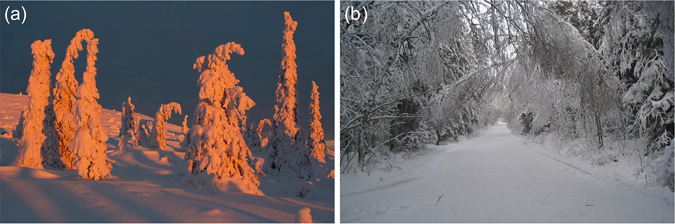
Fig. 12. (a) Spruces heavily loaded by snow and rime in eastern Lapland in January 2014 showing the typical characteristics of the crown snow loads near the alpine timberline. Photo: Teuvo Hietajärvi. (b) Birches bent under heavy crown snow loads in south-western Finland in January 2010. Photo: Ilari Lehtonen.
At least with the G08 method, which does not separate different snow load types and does not take riming into account at all, the dependency of the snow loads on the terrain elevation could not be properly described. The only directly altitude-related dependency in the snow loads simulated by that method can be the decrease of the loads with increasing altitude due to the enhanced wind removal of snow. While temperature conditions at high elevations are often more suitable for snow accretion, the G08 method still seems to produce, on average, the heaviest snow loads over the highest areas (Fig. 6b). The capability of the G08 method to model reasonably the crown snow loads was illustrated by Gregow et al. (2008). They compared the simulated snow loads at Rovaniemi and Sodankylä in Lapland during the winter of 1993/94. The simulated loads were substantially heavier in Sodankylä than in Rovaniemi, because wind speeds were generally higher in Rovaniemi. That is because the measurement site in Rovaniemi is more open and is located at a higher elevation than the one in Sodankylä, especially when compared to the surrounding areas. In Sodankylä, the simulated snow loads were heavy until late February and Gregow et al. (2008) therefore concluded that the G08 method provided reasonable results since the winter is known for widespread snow-induced forest damage in Lapland. However, in Rovaniemi, the crown snow loads were virtually entirely blew away by wind by that time based on the G08 method. In reality, the crown snow loads were very heavy still in March and particularly at high altitudes (Jalkanen and Konôpka 1998). Hence, it is evident that the G08 method would have been unable to simulate the heavy crown snow loads reported by Jalkanen and Konôpka (1998) in March 1994 in the Kivalo research area near Rovaniemi, as this site is located at an even higher altitude than the weather measurement station in Rovaniemi, and the area most likely consequently experiences even higher wind speeds. Nonetheless, based on our results, the FMI model did not prove to perform any better in simulating the heavy crown snow loads during that winter in the area. One possible reason for this is that the accumulation of ice related to a freezing rain event in November 1993 had bent the tree tops south-west, thereby promoting further accumulation of snow later in winter (Jalkanen and Konôpka 1998).
Hoarfrost accumulation is particularly enhanced when the surface is colder than air. Because of this, crown snow loads increase most effectively when weather quickly becomes milder and more humid. Then, all surfaces, including tree branches, might still be colder than the dew point of air and humidity is effectively transformed into hoarfrost. This effect is not directly included in the model calculations, although riming is possible in the FMI model until the air temperature exceeds 1 °C.
Compared to the previous study of Gregow et al. (2008) where the G08 method was applied to study the spatial patterns of heavy crown snow loads in Finland, the more sophisticated FMI model suggested, on average, somewhat heavier snow loads. Moreover, the area with the heaviest snow loads is centred in eastern rather than northern Finland, although the G08 method also produces usually heavier snow loads in the eastern rather than the western parts of the country. Overall, the results accord well with the statement of Solantie (1994) that the region of Kainuu is the area most prone to snow damage in Finland.
Gregow et al. (2008) furthermore proposed that the risk for heavy snow loads had been increasing after the 1960s. This conclusion could not be confirmed in this study, although we noted that wintertime temperature, precipitation and probably relative humidity as well have all manifested increasing trends during the last half of the century. Inhomogeneity in wind speed measurements severely hampered the evaluation of trends in the crown snow loads and though Gregow et al. (2008) performed corrections to the original wind speed measurements, it is unclear whether the procedure produced truly homogeneous wind data. Nevertheless, they concluded that the claimed increase in the occurrence of heavy snow loads resulted at least partly because of the weakening of winds in the 1990s. It is further noteworthy that the stations with no significant wind speed trend in this study are concentrated in southern and western Finland. Moreover, the observed increasing trend in wintertime precipitation, which should result in increasing crown snow loads, is possibly partly artificial, caused by changes in the precipitation gauges in the 1980s. In any case, Kilpeläinen et al. (2010) projected that the risk for snow-induced forest damage in Finland would decrease a little, though not very significantly, already during the period of 1991–2020 when compared to the period 1961–1990. Our results do not suggest that this kind of reduction in the risk would have either occurred by 2010.
7 Conclusions
We have introduced the model used to predict heavy crown snow loads at FMI and produced a description of the spatial variability of the heavy snow loads in Finland with the help of this model. The snow load is divided into rime, dry snow, wet snow and frozen snow within this study. In addition, the results are compared to those received with a simpler method presented previously by Gregow et al. (2008). Based on our results, the heaviest crown snow loads occur, on average, in eastern Finland. Some geographical differences exist in the occurrence of different snow load types, but for every type, the areas with the heaviest loads are found from the eastern parts of the country. This is despite the fact that weather conditions most favourable for riming occur most frequently in the interior of western Finland apart from the hills and fells in the north.
Both for rapid snow load accretion, which is typically related to wet snow, and especially for heavy riming, seasonal distribution peaks in early winter. In northern Finland, conditions are most favourable for heavy snow and rime loading in October, and in southern Finland from November to January. During late winter and spring, heavy riming is very rare except on fells in Lapland but relatively large increases in the total snow load become slightly more common again when the temperature, on average, crosses 0°C in spring.
Over the period from 1961–2010, we could not detect any clear trends in the crown snow load amounts. However, studying the trends was difficult because of inaccuracies related to wind speed measurements. These inaccuracies further somewhat inflicted studying the spatial distribution of the heavy snow loads. Otherwise, the relatively small number of stations that could be included into the analyses restricted the accuracy of the results. However, we could select a wider set of stations than Gregow et al. (2008), as we also accepted all of the stations where precipitation was measured only once a day. As we demonstrated that, on average, the results change only a little, even if hourly precipitation observations are used, we do not believe that the use of 24-hour precipitation sums instead of 12-hour sums that were used by Gregow et al. (2008) would have had any notable effect on the results. In addition, we studied the effect of solar radiation in the results applying the FMI model and found that based on the model results, crown snow loads are decreased due to solar radiation only in late winter and spring, most substantially in March. Hence, we could, in fairly good conscience, omit the effect of solar radiation as this variable is obtainable only from a few stations.
Furthermore, we noted that the crown snow-load values calculated with the daily means of needed weather variables as input, as has been done in some previous studies where the effect of climate change on the crown snow loads have been evaluated, are on average overestimated but have usually some resemblance to the values calculated with hourly input data. Nonetheless, some indirect measures of conditions favourable for snow and rime loading can be also utilised in assessing the risk for snow damage if only the daily means of weather variables are available.
In the future, the FMI model could be improved in several ways. Firstly, the rime load in the model could be divided into soft rime and hard rime as these two rime types have fairly distinct characteristics. For example, soft rime is much more easily removed due to wind as compared to more tightly attached hard rime. This more detailed classification would probably increase the model performance, particularly in the areas where riming is the main cause for crown snow loads and high wind speeds occur frequently. Moreover, the formation of glaze due to freezing rain and the formation of hoarfrost could be included in the model. However, a thorough measurement campaign to measure actual snow loads on trees would be required to comprehensively improve the model parameters. So far, the FMI model has proved to provide satisfactory results in predicting the heavy crown snow loads.
Acknowledgments
Development of the crown snow load model of FMI is based on the work of Reijo Solantie, Mika Heiskanen, Kari Ahti, Bengt Tammelin and Kristiina Säntti. Nea Kuusinen and Frank Berninger from the Department of Forest Sciences, University of Helsinki, are acknowledged for providing the canopy snow classification data. Petri Keronen and Pasi Kolari are acknowledged for processing the SMEAR data. Henriikka Simola is thanked for extracting the weather data from the database of the Finnish Meteorological Institute. Climate Prediction Center of National Center for Environmental Prediction is acknowledged for the NAO data that was provided from their web site at http://www.cpc.ncep.noaa.gov/. This study has been supported by the Academy of Finland through the ADAPT research project (no. 260785). The two anonymous reviewers are acknowledged for their assistance in improving the paper.
References
Aalto J., Pirinen P., Heikkinen J., Venäläinen A. (2013). Spatial interpolation of monthly climate data for Finland: comparing the performance of kriging and generalized additive models. Theoretical and Applied Climatology 112: 99–111. http://dx.doi.org/10.1007/s00704-012-0716-9.
Ahti K. (1978). Huurteen muodostumiseen ja määrään vaikuttavista tekijöistä Suomessa. MSc thesis, University of Helsinki, Helsinki. 31 p. [In Finnish].
Ahti K., Makkonen L. (1982). Observations on rime formation in relation to routinely measured meteorological parameters. Geophysica 19: 75–85.
Baranowski S., Liebersbach J. (1977). The intensity of different kinds of rime on the upper tree line in the Sudety Mountains. Journal of Glaciology 19: 489–497.
Bauer D. (1973). Snow accretion on power lines. Atmosphere 11: 88–96. http://dx.doi.org/10.1080/00046973.1973.9648351.
Bonelli P., Lacavalla M, Marcacci P., Mariani G., Stella G. (2011). Wet snow hazard for power lines: a forecast and alert system applied in Italy. Natural Hazards and Earth System Sciences 11: 2419–2431. http://dx.doi.org/10.5194/nhess-11-2419-2011.
Drage M.A., Hauge G. (2008). Atmospheric icing in a coastal mountainous terrain. Measurements and numerical simulations, a case study. Cold Regions Science and Technology 53: 150–161. http://dx.doi.org/10.1016/j.coldregions.2007.12.003.
ECMWF (2014). http://www.ecmwf.int/products/data/operational_system/. [Cited 21 January 2014].
Goovaerts P. (1997). Geostatistics for natural resources evaluation. Oxford University Press, New York. 483 p.
Gregow H., Peltola H., Laapas M., Saku S., Venäläinen A. (2011). Combined occurrence of wind, snow loading and soil frost with implications for risks to forestry in Finland under the current and changing climatic conditions. Silva Fennica 45: 35–54. http://dx.doi.org/10.14214/sf.30.
Gregow H., Puranen U., Venäläinen A., Peltola H., Kellomäki S., Schultz D. (2008). Temporal and spatial occurrence of strong winds and large snow load amounts in Finland during 1961–2000. Silva Fennica 42: 515–534. http://dx.doi.org/10.14214/sf.231.
Häggmark L., Ivarsson K.-I., Gollvik S., Olofsson P.-O. (2000). Mesan, an operational mesoscale analysis system. Tellus 52A: 2–20.
Hari P., Kulmala M. (2005). Station for measuring ecosystem–atmosphere relations (SMEAR II). Boreal Environment Research 10: 315–322.
Heikinheimo O. (1920). Suomen lumituhoalueet ja niiden metsät. Metsätieteellisen koelaitoksen julkaisuja 3. [In Finnish].
Hlásny T., Křístek Š., Holuša J., Trombik J., Urbaňcová N. (2011). Snow disturbances in secondary Norway spruce forests in Central Europe: regression modeling and its implications for forest management. Forest Ecology and Management 262: 2151–2161. http://dx.doi.org/10.1016/j.foreco.2011.08.005.
Hofstra N., Haylock M., New M., Jones P., Frei C. (2008). Comparison of six methods for the interpolation of daily, European climate data. Journal of Geophysical Research 113: D21110. http://dx.doi.org/10.1029/2008JD010100.
Holton J.R. (2004). An introduction to dynamic meteorology, 4th ed. Elsevier Academic Press, New York, London. 535 p.
Homola M.C., Virk M.S., Nicklasson P.J., Sundsbø P.A. (2012). Performance losses due to ice accretion for a 5 MW wind turbine. Wind Energy 15: 379–389. http://dx.doi.org/10.1002/we.477.
Jalkanen A., Mattila U. (2000). Logistic regression models for wind and snow damage in northern Finland based on the National Forest Inventory data. Forest Ecology and Management 135: 315–330. http://dx.doi.org/10.1016/S0378-1127(00)00289-9.
Jalkanen R., Konôpka B. (1998). Snow-packing as a potential harmful factor on Picea abies, Pinus sylvestris and Betula pubescens at high altitude in northern Finland. European Journal of Forest Pathology 28: 373–382. http://dx.doi.org/10.1111/j.1439-0329.1998.tb01191.x.
Junninen H., Lauri A., Keronen P., Aalto P., Hiltunen V., Hari P., Kulmala M. (2009). Smart-SMEAR: on-line data exploration and visualization tool for SMEAR stations. Boreal Environment Research 14: 447–457.
Kilpeläinen A., Gregow H., Strandman H., Kellomäki S., Venäläinen A., Peltola H. (2010). Impacts of climate change on the risk of snow-induced forest damage in Finland. Climatic Change 99: 193–209. http://dx.doi.org/10.1007/s10584-009-9655-6.
Kuusinen N., Kolari P., Levula J., Porcar-Castell A., Stenberg P., Berninger F. (2012). Seasonal variation in boreal pine forest albedo and effects of canopy snow on forest reflectance. Agricultural and Forest Meteorology 164: 53–60. http://dx.doi.org/10.1016/j.agrformet.2012.05.009.
Lahti K., Lahtinen M., Nousiainen K. (1997). Transmission line corona losses under hoar frost conditions. IEEE Transactions on Power Delivery 12: 928–933. http://dx.doi.org/10.1109/61.584415.
Lomilina L.E. (1977). The effect of relief on glaze-ice and rime deposition. Soviet Meteorology and Hydrology 2: 49–55.
Makkonen L. (1981). Estimating intensity of atmospheric ice accretion on stationary structures. Journal of Applied Meteorology 20: 595–600. http://dx.doi.org/10.1175/1520-0450(1981)020<0595:EIOAIA>2.0.CO;2.
Makkonen L. (1984). Modeling of ice accretion on wires. Journal of Climate and Applied Meteorology 23: 929–939. http://dx.doi.org/10.1175/1520-0450(1984)023<0929:MOIAOW>2.0.CO;2.
Makkonen L. (1989). Estimation of wet snow accretion on structures. Cold Regions Science and Technology 17: 83–88. http://dx.doi.org/10.1016/S0165-232X(89)80018-7.
Makkonen L. (2000). Models for the growth of rime, glaze icicles and wet snow on structures. Philosophical Transactions of the Royal Society of London, Series A 358: 2913–2939. http://dx.doi.org/10.1098/rsta.2000.0690.
Makkonen L. (2013). A model of hoarfrost formation on a cable. Cold Regions Science and Technology 85: 256–260. http://dx.doi.org/10.1016/j.coldregions.2012.10.001.
Makkonen L., Ahti K. (1995). Climatic mapping of ice loads based on airport weather observations. Atmospheric Research 36: 185–193. http://dx.doi.org/10.1016/0169-8095(94)00034-B.
Makkonen L., Laakso T. (2005). Humidity measurements in cold and humid environments. Boundary-Layer Meteorology 116: 131–147. http://dx.doi.org/10.1007/s10546-004-7955-y.
Makkonen L., Wichura B. (2010). Simulating wet snow loads on power line cables by a simple model. Cold Regions Science and Technology 61: 73–81. http://dx.doi.org/10.1016/j.coldregions.2010.01.008.
Marchand P. (1987). Life in cold. An introduction to winter ecology. University Press, London. 320 p.
Martiník A., Mauer O. (2012). Snow damage to birch stands in Northern Moravia. Journal of Forest Science 58: 181–192.
McKay G.A., Thompson H.A. (1969). Estimating the hazard of ice accretion in Canada from climatological data. Journal of Applied Meteorology 8: 927–935. http://dx.doi.org/10.1175/1520-0450(1969)008<0927:ETHOIA>2.0.CO;2.
Nock C.A., Greene D., Delagrange S., Follett M., Fournier R., Messier C. (2013). In situ quantification of experimental ice accretion on tree crowns using terrestrial laser scanning. PLoS ONE 8: e64865. http://dx.doi.org/10.1371/journal.pone.0064865.
Nygaard B.E.K., Ágústsson H., Somfalvi-Tóth K. (2013). Modeling wet snow accretion on power lines: improvements to previous methods using 50 years of observations. Journal of Applied Meteorology and Climatology 52: 2189–2203. http://dx.doi.org/10.1175/JAMC-D-12-0332.1.
Nykänen M.-L., Peltola H., Quine C.P., Kellomäki S., Broadgate M. (1997). Factors affecting snow damage of trees with particular reference to European conditions. Silva Fennica 31: 193–213.
Päätalo M.-L. (2000). Risk of snow damage in unmanaged and managed stands of Scots pine, Norway spruce and birch. Scandinavian Journal of Forest Research 15: 530–541. http://dx.doi.org/10.1080/028275800750173474.
Päätalo M.-L., Peltola H., Kellomäki S. (1999). Modelling the risk of snow damage to forests under short-term snow loading. Forest Ecology and Management 116: 51–70. http://dx.doi.org/10.1016/S0378-1127(98)00446-0.
Peltola H., Nykänen M.-L., Kellomäki S. (1997). Model computations on the critical combination of snow loading and windspeed for snow damage of scots pine, Norway spruce and Birch sp. at stand edge. Forest Ecology and Management 95: 229–241. http://dx.doi.org/10.1016/S0378-1127(97)00037-6.
Peltola H., Kellomäki S., Väisänen H., Ikonen V.-P. (1999). A mechanistic model for assessing the risk of wind and snow damage to single trees and stands of Scots pine, Norway spruce, and birch. Canadian Journal of Forest Research 29: 647–661. http://dx.doi.org/10.1139/x99-029.
Petty J.A., Worrell R. (1981). Stability of coniferous tree stems in relation to damage by snow. Forestry 54: 115–128. http://dx.doi.org/10.1093/forestry/54.2.115.
Ruosteenoja K., Jylhä K., Mäkelä H., Hyvönen R., Pirinen P., Lehtonen I. (2013). Rakennusfysiikan testivuosien sääaineistot havaitussa ja arvioidussa tulevaisuuden ilmastossa – REFI-B-hankkeen loppuraportti. Finnish Meteorological Institute, Reports 2013:1. 48 p. [In Finnish with English abstract].
Rustad L.E., Campbell J.L. (2012). A novel ice storm manipulation experiment in a northern hardwood forest. Canadian Journal of Forest Research 42: 1810–1818. http://dx.doi.org/10.1139/x2012-120.
Ryerson C.C. (1990). Atmospheric icing rates with elevation on northern New England mountains, U.S.A. Arctic and Alpine Research 22: 90–97.
Sakamoto Y. (2000). Snow accretion on overhead wires. Philosophical Transactions of the Royal Society of London, Series A 358: 2941–2970. http://dx.doi.org/10.1098/rsta.2000.0691.
Schelhaas M.-J., Nabuurs G.-J., Schuck A. (2003). Natural disturbances in the European forests in the 19th and 20th centuries. Global Change Biology 9: 1620–1633. http://dx.doi.org/10.1046/j.1365-2486.2003.00684.x.
Seidl R., Fernandes P.M., Fonseca T.F., Gillet F., Jönsson A.M., Merganičová K., Netherer S., Arpaci A., Bontemps J.-D., Bugmann H., González-Olabarria J.R., Lasch P., Meredieu C., Moreira F., Schelhaas M.-J., Mohren F. (2011). Modelling natural disturbances in forest ecosystems: a review. Ecological Modelling 222: 903–924. http://dx.doi.org/10.1016/j.ecolmodel.2010.09.040.
Sevola Y. (ed.). (1999). Finnish Statistical Yearbook of Forestry. Finnish Forest Research Institute, Helsinki. 352 p.
Solantie R. (1994). Effect of weather and climatological background on snow damage of forests in Southern Finland in November 1991. Silva Fennica 28: 203–211.
Sugiura K., Ohata T., Yang D. (2006). Catch characteristics of precipitation gauges in high-latitude regions with high winds. Journal of Hydrometeorology 7: 984–994. http://dx.doi.org/10.1175/JHM542.1.
Tammelin B., Säntti K. (1998). Icing in Europe. In: Proceedings of the International Conference, Wind Energy Production in Cold Climate, Boreas IV, 31 March – 2 April 1998, Hetta, Finland, Finnish Meteorological Institute. p. 125–132.
Thorkildson R.M., Jones K.F., Emery M.K. (2009). In-cloud icing in the Columbia basin. Monthly Weather Review 137: 4369–4381. http://dx.doi.org/10.1175/2009MWR2941.1.
Undén P., Rontu L., Järvinen H., Lynch P., Calvo J., Cats G., Cuxart J., Eerola K., Fortelius C., Garcia-Moya J.A., Jones C., Lenderlink G., McDonald A., McGrath R., Navascues B., Nielsen N.W., Ødegaard V., Rodriguez E., Rummukainen M., Rõõm R., Sattler K., Sass B.H., Savijärvi H., Schreur B.W., Sigg R., The H., Tijm A. (2002). HIRLAM-5 scientific documentation. Swedish Meteorological and Hydrological Institute, Norrköping. 144 p.
Vajda A., Venäläinen A. (2003). The influence of natural conditions on the spatial variation of climate in Lapland, northern Finland. International Journal of Climatology 23: 1011–1022. http://dx.doi.org/10.1002/joc.928.
Valinger E., Fridman J. (1997). Modelling probability of snow and wind damage in Scots pine stands using tree characteristics. Forest Ecology and Management 97: 215–222. http://dx.doi.org/10.1016/S0378-1127(97)00062-5.
Valinger E, Fridman J. (1999). Models to assess the risk of snow and wind damage in pine, spruce, and birch forests in Sweden. Environmental Management 24: 209–217. http://dx.doi.org/10.1007/s002679900227.
Valinger E., Lundqvist L. (1992). The influence of thinning and nitrogen fertilisation on the frequency of snow and wind induced stand damage in forests. Scottish Forestry 46: 311–320.
Valinger E., Lundqvist L., Bondesson L. (1993). Assessing the risk of snow and wind damage from tree physical characteristics. Forestry 66: 249–260. http://dx.doi.org/10.1093/forestry/66.3.249.
Valinger E., Lundqvist L., Brandel G. (1994). Wind and snow damage in a thinning and fertilisation experiment in Pinus sylvestris. Scandinavian Journal of Forest Research 9: 129–134. http://dx.doi.org/10.1080/02827589409382822.
Vastaranta M., Korpela I., Uotila A., Hovi A., Holopainen M. (2012). Mapping of snow-damaged trees based on bitemporal airborne LiDAR data. European Journal of Forest Research 131: 1217–1228. http://dx.doi.org/10.1007/s10342-011-0593-2.
Visbeck M.H., Hurrell J.W., Polvani L., Cullen H.M. (2001). The North Atlantic Oscillation: past, present, and future. Proceedings of the National Academy of Sciences of the United States of America 98: 12876–12877. http://dx.doi.org/10.1073/pnas.231391598.
Wang S., Jiang X. (2012). Progress in research on ice accretion on overhead transmission lines and its influence on mechanical and insulating performance. Frontiers of Electrical and Electronic Engineering 7: 326–336. http://dx.doi.org/10.1007/s11460-012-0197-8.
Yang D., Goodison B.E., Metcalfe J.R., Louie P., Leavesley G., Emerson D., Hanson C.L., Golubev V.S., Elomaa E., Gunther T., Pangburn T., Kang E., Milković J. (1999). Quantification of precipitation measurement discontinuity induced by wind shields on national gauges. Water Resources Research 35: 491–508. http://dx.doi.org/10.1029/1998WR900042.
Zavarina M.V., Lomilina L.G. (1976). Der Einfluß des Reliefs und der Seehöhe des Ortes auf die Größe der Eislasten. Zeitschrift für Meteorologie 26: 105–106. [In German].
Zhou Y., Niu S., Lü J., Zhao L. (2013). Meteorological conditions of ice accretion based on real-time observation of high voltage transmission line. Chinese Science Bulletin 57: 812–818. http://dx.doi.org/10.1007/s11434-011-4868-2.
Zubizarreta-Gerendiain A., Pellikka P., Garcia-Gonzalo J., Ikonen V.-P., Peltola H. (2012). Factors affecting wind and snow damage of individual trees in a small management unit in Finland: assessment based on inventoried damage and mechanistic modelling. Silva Fennica 46: 181–196. http://dx.doi.org/10.14214/sf.441.
Total of 69 references
Appendix A
Appendix A, Description of the crown snow load model of FMI, is available at http://www.silvafennica.fi/supp_files/article1120/appendix.pdf.
