Joanna Bachmatiuk  ,
Jordi Garcia-Gonzalo,
Jose Guilherme Borges
,
Jordi Garcia-Gonzalo,
Jose Guilherme Borges
Analysis of the performance of different implementations of a heuristic method to optimize forest harvest scheduling
Bachmatiuk J., Garcia-Gonzalo J., Borges J. G. (2015). Analysis of the performance of different implementations of a heuristic method to optimize forest harvest scheduling. Silva Fennica vol. 49 no. 4 article id 1326. https://doi.org/10.14214/sf.1326
Highlights
- The number of treatment schedules available for each stand has an impact on the optimal configuration of opt-moves (i.e. number stands where the treatment schedule is changed in an iteration)
- Considering a large number of treatment schedules per stand, the one-opt move implementation is preferred, yet when considering a low number of decision choices the two-opt moves option performs better.
Abstract
Finding an optimal solution of forest management scheduling problems with even flow constraints while addressing spatial concerns is not an easy task. Solving these combinatorial problems exactly with mixed-integer programming (MIP) methods may be infeasible or else involve excessive computational costs. This has prompted the use of heuristics. In this paper we analyze the performance of different implementations of the Simulated Annealing (SA) heuristic algorithm for solving three typical harvest scheduling problems. Typically SA consists of searching a better solution by changing one decision choice in each iteration. In forest planning this means that one treatment schedule in a single stand is changed in each iteration (i.e. one-opt move). We present a comparison of the performance of the typical implementation of SA with the new implementation where up to three decision choices are changed simultaneously in each iteration (i.e. treatment schedules are changed in more than one stand). This may allow avoiding local optimal. In addition, the impact of SA - parameters (i.e. cooling schedule and initial temperature) are tested. We compare our heuristic results with a MIP formulation. The study case is tested in a real forest with 1000 stands and a total of 213116 decision choices. The study shows that when the combinatorial problem is very large, changing simultaneously the treatment schedule in more than one stand does not improve the performance of SA. Contrarily, if we reduce the size of the problem (i.e. reduce considerably the number of alternatives per stand) the two-opt moves approach performs better.
Keywords
harvest scheduling;
simulated annealing;
heuristic;
cooling schedule;
initial temperature
-
Bachmatiuk,
Centro de Estudos Florestais, Instituto Superior de Agronomia, Universidade de Lisboa, Lisboa, Portugal
E-mail
jbachmatiuk@isa.ulisboa.pt
- Garcia-Gonzalo, Centro de Estudos Florestais, Instituto Superior de Agronomia, Universidade de Lisboa, Lisboa, Portugal E-mail jordigarcia@isa.ulisboa.pt
- Borges, Centro de Estudos Florestais, Instituto Superior de Agronomia, Universidade de Lisboa, Lisboa, Portugal E-mail joseborges@isa.ulisboa.pt
Received 27 February 2015 Accepted 3 June 2015 Published 7 July 2015
Views 108044
Available at https://doi.org/10.14214/sf.1326 | Download PDF

1 Introduction
In many cases considering harvest scheduling problem in forestry implies taking into account sustainability constraints together with the need to preserve wildlife habitat and to maintain aesthetic aspects. In addition, addressing sustainability concerns in forest planning requires to take into account the spatial distribution of harvests to meet spatial objectives. For example, sometime it will be needed to use adjacency constraints (i.e. the harvested area of adjacent management units within or between periods is limited to a maximum size) to limit the maximum size of an open (clear-cut) area. In this context harvest scheduling problems are a challenge as these models represent complex combinatorial problems that may be hard and complex to solve.
The main approaches to represent adjacency constraints in forest management were described by Murray (1999). Two fundamental methodologies have been introduced in order to incorporate those constraints into a forest management model. The first approach, the Unit Restriction Model (URM), does not allow harvesting two adjacent management units during one period or green-up period (regardless of size), thus the unit restrictions arrangement are represented by pairwise adjacency constraints. This formulation assumes that a simple management unit encompasses the area close to the maximum opening size. The second approach of defining adjacency constraints is the Area Restriction Model (ARM), which for modeling allows scheduling contiguous management units if the total size of the clear-cut area does not exceed the maximum opening size that is assumed. However, from the computation point, ARM approach is difficult to formulate and solve, due to the complexity of imposing the relationship of given management unit to the others units as well as their contiguous units.
The URM has been solved both by mathematical programming (e.g. Snyder and Revelle 1996), by heuristic approaches (e.g. Nelson and Brodie 1990) and by combinations of both (e.g. Borges and Hoganson 2000). Research has been conducted to increase the efficiency of the solution of the more general case of ARM. For instance, McDill et al. (2002) presented the Path Algorithm, which consists of clustering contiguous stands that if cut altogether would exceed the maximum opening size, and then adding a constraint that does not allow to harvest at those clusters. Another formulation proposed consists in defining variables for all possible and feasible harvesting clusters and adding constraints that prevent harvesting adjacent pairs of clusters (McDill et al. 2002; Goycoolea et al. 2005). A third method called the Bucket formulation consists in defining buckets a priori and then assigning stands to each of them so that each bucket represents a harvested cluster (Constantino et al. 2008). For a deeper discussion of these formulations we refer the reader to Goycoolea et al. (2009). Recent work of Tóth et al. (2013) states that the path approach can be further enhanced by using lazy constraints. In this method the path constraints are not active, this is why those constraints are defined as lazy constraint pools, which leads to the amelioration of model in terms of solution time.
Mathematical programming approaches to solve harvest scheduling problems with spatial restrictions cost computational time and may end up with a high optimality gap or without finding a feasible solution (Borges et al. 2002; Zhu et al. 2007). One way to reduce computation time and the amount of memory required is to raise the optimality gap. However, this may lead to poor solutions. Another way would be to improve the existing traditional methods, what has been shown above. Another approach is to use search process such as heuristics.
The heuristics most commonly used in forest planning problems include Simulated Annealing (SA), Tabu Search, and genetic algorithms (Heinonen and Pukkala 2004). SA has attracted significant interest since the publication of Kirkpatrick et al. (1983), which presented the optimization heuristic technique consisting of the idea of physical phenomena such as controlled cooling of a material that was heated well above its known melting point. Simulated Annealing has been extensively used in forest management planning. For example, SA has been applied in harvest scheduling problems including adjacency constraints (Lockwood and Moore 1993). In addition SA has been included in decision support system (DSS) tools (Falcão and Borges 2005).
Most of standard heuristics try to improve the solution gradually by changing it locally, and usually only a little at a time. A new solution may be obtained from the current solution with one move. When referring to harvest scheduling problems a move may consist of changing the treatment schedule in just one management unit (i.e. stand). In this case we may talk about one-opt move solution approach (Reeves 1993; Bettinger et al. 1999; Bettinger et al. 2002). However, a new solution may be obtained by changing the schedule in more than one management unit. Then we may talk about an x – opt moves heuristic with x as a number of moves e.g. change in the treatment schedule in x management units per iteration. In this context, some authors (Bettinger et al. 1999; Bettinger et al. 2002; Heinonen and Pukkala 2004) have analyzed the performance of different heuristic methods (e.g. Random Ascent, Hero, Tabu Search) when implementing different number of changes (one and two) per iteration.
In forestry problems, the performance of the traditional implementations of SA (i.e. one-opt move) has been analyzed and compared to other heuristic methods by Pukkala and Kurttila (2005). Recently a modification of SA has been applied by Borges et al. (2014a, b) where one-opt move implementation was used and different methods to select the unit where the management schedule is changed were evaluated. In addition, Heinonen and Pukkala (2004) studied the efficiency of SA using one and two changes per iteration. In other scientific areas (e.g. vehicle routing) SA has been implementing using more than two changes per iteration (e.g. Alfa et al. 1991; Aarts and Lenstra 2003; Ghaffari-Nasab and Saboury 2013). However, to our best knowledge, the only study in forestry problems analyzing the use of more than two changes was presented by Garcia-Gonzalo et al. (2012). In a preliminary study they compared the performance of SA when using up to three-opt moves in a harvest scheduling planning problem. Although they used the same study area than in our article, they did not include adjacency constraints and used a limited number of management alternatives per unit which made the problem much simpler.
Our study presents a comparison of the performance of a heuristic technique (Simulated Annealing) where different number of moves (i.e. one-opt to three-opt moves) are performed in each iteration to address a very large and complex planning problem including adjacency constraints. Previous works applied in forest planning problems using a small number of decision choices conclude that two-opt move are more effective than one-opt moves (Bettinger et al. 1999; Heinonen and Pukkala 2004). In this study we test if in very large problems (e.g. problems involving several stands with a large number of decision choices per stand) increasing the number of opt-moves (up to three-opt moves) will be more effective than the typical implementation of SA (i.e. one-opt move). For testing purposes these different implementations are applied to different instances (i.e. forest of different sizes) of three real harvest scheduling problems with a large number of available treatment schedules of a Eucalypt plantation. In order to see if results are sensitive to the number of treatment schedules available for each stand, we also solved the biggest problem instance using adjacency constraints and a small number of treatment schedules for each stand. On the other hand we analyze the impact of different SA parameters in the quality of the solution. In order to verify the quality of solution provided by SA, we attempt to solve the problem as mixed integer programming (MIP) by implementing the commercial solver CPLEX.
2 Material and methods
2.1 Problem formulation
The forest planning problem that we investigate involved the maximization of the net present value (NPV) of timber harvested of a forest located in central Portugal (Fig. 1). The eucalypt test forest encompasses 1000 stands and extends over 11873 ha. In this planning problem the manager has to decide which management schedule to apply in each of the stands during the next 30 years. In each treatment schedule, it occurs at least one harvest event. The goal of this study is to harvest each management unit at least once, therefore one treatment schedule must be assigned to management unit. For testing purposes we select smaller areas within the test forest to develop smaller problems.
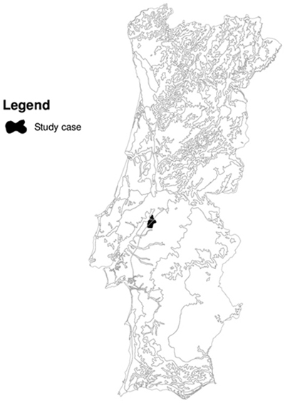
Fig. 1. The map of Portugal and the study area.
In this study, a typical eucalyptus rotation may include up to 2 or 3 coppice cuts, each coppice cut being followed by a stool thinning that may leave on average 1.5 shoots per stool. Harvest ages may range from 9 to 15. Initial density after a plantation may be 1500 trees per ha. Based on these silviculture parameters we constructed possible treatment schedules for each stand in the test forest, over a planning horizon of thirty 1-year periods. In the first experiment (experiment I) all possible combinations of the parameters used in the prescriptions were combined to develop a large set of treatment schedules (i.e. prescriptions). The number of stand treatment schedules ranged from 166 to 278, resulting in 213116 decision choices. In this context, the size of the solution space is large and the problem becomes very complex. Experiment I is at the core of our analysis as we want to test the performance of SA when using a very large number of treatment schedules per stand. In order to test the sensitivity of the comparison of the number of changes per iteration to the number of treatment schedules we developed a smaller planning problem (experiment II). In this case we used the same forest instances but we reduced the planning horizon to 15 years and we selected a fewer number of treatment schedules. In total between 7 and 15 treatment schedules were used for each stand resulting in 12573 decision choices.
A former decision support system (DSS) (Borges et al. 2002; Falcão and Borges 2005) recently updated by Garcia-Gonzalo et al. (2014) was used to quantify the outcomes associated to all treatment schedules (i.e. prescriptions) and stands. The growth estimated by the DSS provides the information needed to assess the impact of each treatment schedule on results and conditions of interest (e.g. volume harvested). Both economic objective (i.e. net present value (NPV) using a 3 percent discounting rate) and timber flows were considered.
Following the model formulation I by Johnson and Scheurmann (1977), the forest management model can be described as:


![]()
![]()
![]()
![]()
![]()

![]()
where
I = the number of stands.
Ji = the number of treatment schedules for stand i.
T = the number of years for a given horizon time.
npvij = net present value associated with treatment schedule j for a stand i.
xij = binary variable which = 1 if treatment schedule j is assigned to the stand i and 0otherwise.
vijt = volume harvested in stand i in year t if treatment schedule j is selected.
Vt = total volume harvested in year t.
![]() = volume of the ending inventory in stand i if treatment schedule j is selected.
= volume of the ending inventory in stand i if treatment schedule j is selected.
![]() = total volume of the ending inventory.
= total volume of the ending inventory.
cijt = average carbon stock in stand i in year t if treatment schedule j is selected.
Ct = total carbon stock in year t.
α = deviation allowed from target level for volume harvest.
β = deviation allowed from target level for carbon.
ϑ = ending inventory goal.
![]() = minimally infeasible cluster representing a contiguous set of stands generated by algorithm proposed by Goycoolea et al. (2009).
= minimally infeasible cluster representing a contiguous set of stands generated by algorithm proposed by Goycoolea et al. (2009).
Λ+ = set of minimally infeasible clusters.
Eq. 1 defines the objective of maximizing net present value (NPV includes the value of the ending inventory). Eq. 2 states that one and only one treatment schedule is assigned to each stand. Eq. 3 is used to count the volume harvested in each year t (accounting row). Eq. 4 calculates the volume of ending inventory (accounting row). Eq. 5 represents the carbon level in each year t (accounting row). Inequalities 6 and 7 define the even flow (maximum of 10% variation among periods) of harvests over the planning horizon that may ensure the sustainability of the forest. Inequality 8 ensures that the ending inventory target is met. Inequalities 9 and 10 express carbon stock level flow over the planning horizon (maximum of 10% variation among periods). Inequality 11 is the Path Inequality (Goycoolea et al. 2009) and ensures that in each period the size of harvested contiguous stands does not exceed the maximum clear-cut opening size. Constraint 12 states the binary requirements on decision choice.
For testing purposes, 3 different problem formulations were tested, where each of the problems was built from the previous formulation adding more constraints. The equations for each problems are given below:
Problem I = Eq. 1–3, 6–7, 12.
Problem II = Eq. 1–10, 12.
Problem III = Eq. 1–12.
Problem I encompassed the use of even-flow of harvest constraints (no ending inventory and carbon stock constraints nor adjacency constraints), Problem II further included the use of ending volume inventory and carbon stock level constraints (no adjacency constraints). Problem III was an extension of previous models and further included adjacency constraints, what make this problem more complex compared to foregoing problems formulations. In experiment I we solved problems I, II and III. Because the number of decision choices in experiment II is small we focused our analysis in problem III, which is more difficult to solve.
2.2 Methods
Linear and mixed integer programming have been widely used to obtain a global optimal solution. The main advantage of using them is that when a solution is found one is confident that this is the optimal solution (or optimal with a minor tolerance). However, as explained by Bettinger et al. (2009), their main limitations are (1) the inability to solve some problems in a reasonable amount of time, and (2) a limit on the number of rows (constraints) or variables that can be included in a problem. Of course these limitations are becoming less problematic as model building and computer technology evolves. However, they remain as an important problem.
For example, Murray and Weintraub (2002) illustrated a case where a significant amount of time was required to generate the constraints for a relatively small spatially-constrained problem. Even if McDill and Braze (2001) presented a number of cases, where exact integer solutions (with small tolerance gaps) were obtained in a reasonable amount of time and yet they suggested that alternatives to exact approaches may still be needed. In fact, Bertomeu and Romero (2001) and Murray and Weintraub (2002) suggested that it may be unrealistic to solve large or difficult problems with exact approaches. Thus, for solving large problems or very complex problems when mathematical programming methods become impractical, researchers have been exploring alternatives to search processes, (.e.g. when addressing spatial harvest scheduling forest planning problems). One alternative may be the use of heuristic methods which are search processes that apply logical strategies and rules which provides satisfactory results in a reasonable time. However, there is no guarantee, that the best solution located is the global optimum solution. The pertinence of choosing heuristics is presented by Pukkala and Kurttila (2005). In addition, heuristics are more promising, than classical methods, due to its better accommodation to complex planning problems encompassing spatial concerns (Bettinger and Kim 2008).
In order to solve the decision problem presented in subsection 2.1 we use a meta-heuristic called Simulated Annealing (SA) because it is one of the most used heuristic methods. Further different implementations of this heuristic techniques are analyzed.
2.2.1 Simulated Annealing
The first implementation of SA in optimization was proposed by Kirkpatrick et al. (1983) and emanates from Metropolis et al. (1953). This method mimics the annealing physical process by simulating a process of cooling a material that was heated well above its known melting point (initial temperature T0 ), until the system is frozen. Cooling is controlled by cooling schedule parameter, and refers to the geometrical decrement:
where
ζ ˂ 1 and
Tt = temperature at iteration t, where t = 1, 2,..., n, and n is a number of iterations.
Usually in the literature ζ is close to 1 but not lower than 0.8 (Heinonen and Pukkala 2004).
The algorithm at first searches for a good local optimum solution by accepting worse moves with a probability according to the Metropolis criteria. In addition to the cooling schedule parameter, initial temperature has also an impact in the acceptance of an inferior solution. The lower the initial temperature, the higher probability of rejecting the worse solution according to the Metropolis criteria.
The heuristic allows finding a near optimal solution to the problem with a relatively short simulation time. SA involves a sequence of iterations each consisting of randomly changing the current solution to find a new solution in the neighborhood of the current solution (Pham and Karaboga 2000).
In order to avoid premature convergence to a local optimum, an inferior solution may be accepted. This is a fundamental property of metaheuristics because it allows for a more extensive search for the optimal solution. Yet, the frequency of these moves decreases with the iteration number according to the value of a control parameter (temperature) (Reeves 1993). A candidate solution is generated at each iteration. If the current solution is better than the best solution found so far, it replaces the latter. If not, the inferior solution may be accepted and the search process moves forward. The probability of doing so is directly dependent on the temperature and is given by following formula known as Metropolis criteria (Pham and Karaboga 2000):
where:
Dij = the value of objective function of selected solution pi minus the value of objective function of the best solution found so far pj.
The probability of accepting inferior solutions decreases with temperature decreases, and it also decreases with the magnitude with larger differences between the objective function values of the proposed and the best solutions.
Key to successful algorithm implementation is the choice regarding the solution data structure, the fitness evaluation function and the cooling schedule (Pham and Karaboga 2000). In general, the latter involves the specification of the initial temperature parameter, of the rate at which the temperature is reduced and of the number of iterations at each temperature.
The algorithm shown below describes Simulated Annealing search process.
Algorithm Simulated Annealing:
begin
Initialization: T0 - initial temperature, n - number of iterations, ζ - cooling rate,
pj - initial treatment schedule.
Pbest = pj
T = T0
for i = : 1 to n do
pi =change_current_treatment_schedule(pj ) Dij = Value[pi ]- Value[pj ]
if Dij > 0do
pj = pi
if Value[pi]> Value[pbest] do
pbest = pi
else
if ![]() ≥ random(0,1) do
≥ random(0,1) do
pj = pi
Tt = ζ× Tt–1
end
2.2.2 Experimental Design
In this study the heuristic technique (Simulated Annealing) was used to solve the harvest scheduling problems presented in current section. The first objective of the article was to compare the efficiency of the technique when increasing the number of opt-moves (from one to three). By increasing the number of opt-moves, the treatment schedule is changed in more than one stand simultaneously in each iteration. Two experiments were developed differing in the size of the final problems to solve. In experiment I we solved three problems defined in Section 2 for a planning problem covering a 30 years planning horizon. In this experiment a large number of treatment schedules are available (up to 278). In experiment II, we reduced the size of the planning problem to address by decreasing the planning horizon and the number of treatment schedules available for each stand. In this case, only the problem III (i.e. the most complicated due to the use of adjacency constraints) presented in section 2 was solved for a planning horizon of 15 years (1-year period) and with a small number of treatment schedules (i.e. up to 15). Since the objective of the second experiment is to analyze if the number of treatment schedules available has an impact on the optimal number of changes per move and the amount of decision choices is small to address, only problem III (the most complex to solve) is analyzed in detail.
Heuristics are sensitive to the parameters used (Pukkala and Heinonen 2006). Thus a second goal of this article was to analyze the impact of different SA parameters in the quality of the solutions found. This was used to parameterize SA for later comparisons with the MIP solver (i.e. CPLEX). For this purpose we tested different values of the cooling schedule parameter and the initial temperature. All parameters that are mentioned below were chosen based on the experience in Falcão and Borges (2002), as well as on several trial and error runs of the search process.
In this context we used two different values of the cooling schedule parameter. Comparing small and high values allowed us to verify, whether it is recommended to accept inferior solutions at the beginning of the search process and then only search for improvement near local optimum or whether it is appropriate to decelerate the cooling process and accept inferior solutions during more iterations.
In this article we used the following cooling schedule parameters:
ζ1 = 0.8
ζ2 = 0.99996
For the initial temperature the following values were tested:
T0 = {2, 7, 12, 100, 100000}
To evaluate the methods of SA parameters resolution we tested our models on several instances that varied according to the number of stands. The experimental instances included 100, 250, 500, and 1000 stands, taken from the real instance (1000 stands) at random, considering a group of 3 problems formulations stated in Section 2. All of them included the complete forest data, without any relaxation from the original formulation. Moreover, to better evaluate the performance of heuristic, we compared the solution to the solution from MIP solver.
Numerical experiments were carried out in a computer with following features:
Core: Intel i5 650
RAM Memory: 6 GB
OS: WIN 8.1 Pro 64 Bits
CPLEX: Version 12.5.1.0 64 Bits
PYTHON: Version 2.7 64 Bits
3 Results
3.1 Impact on the heuristic solution of the parameters used
The application of heuristic methods involves the testing of convergence and evaluation of parameters (Falcão and Borges 2002). In order to assess the impact on the heuristic solution of the parameters used in SA we solved the planning problems presented in section 2 using all combinations of initial temperature, cooling schedule and number of changes per iteration; in total 30 test computer runs for each problem instance analyzed were performed.
The quality of the solutions provided by SA differed depending on the problem, instance and parameters used. The SA was particularly sensitive to the number of iterations which was chosen based on several trial and error runs of the search process. Due to the size of the defined problem, it was difficult to find a good solution with a small number of iterations. Our goal was to obtain a solution within a maximum gap of 3% compared to the best solution found by CPLEX. Consequently the search process encompassed 300000 iterations. In fact, using a higher number of iterations did not show improvement and the same solutions were obtained. As an example of feasible solution we show the harvest schedule generated by SA for periods 1, 10, 20 and 30 (Fig. 2).
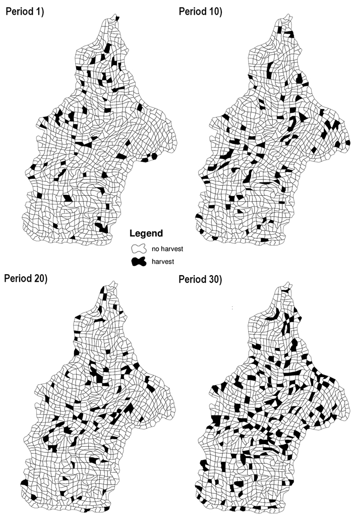
Fig. 2. Maps of study case area presenting harvest schedule generated by Simulated Annealing (SA) for problem III. Stands in black are harvested stands in the corresponding period. Problem III corresponded to the maximization of net returns using even-flow of harvest constraints, ending volume inventory and carbon stock level constraints and adjacency constraints.
3.1.1 Experiment I
Results show that regardless of the problem solved (Problems I, II and III), the initial temperature and cooling schedule, when using a high number of treatment schedules, one-opt move implementation of the SA achieved a better solution than the two-opt and three-opt moves implementations (Fig. 3). In addition performing more changes per iteration increased the solution time and for smaller instances (100 and 250 stands) they were not able to find feasible solutions. Therefore to show the effect of initial temperature and cooling schedule we only present the impacts on the SA implementation using one-opt move.
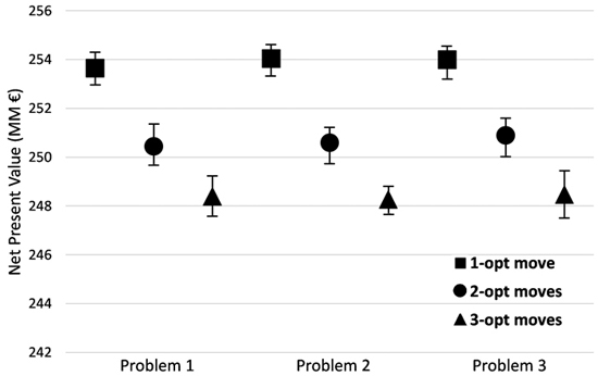
Fig. 3. Performance of the different implementations of Simulated Annealing (SA) (one, two and three-opt moves) for all problem formulations and for the instance of 1000 stands for different combinations of initial temperature (2, 7, 12, 100, 100000) and cooling schedule (0.8, 0.99996). The graph shows the best, the average and the worst solution for each implementation problem. Problem I encompassed the use of even-flow of harvest constraints, Problem II further included the use of ending volume inventory and carbon stock level constraints. Problem III was an extension of previous models and further included adjacency constraints.
After a series of experiments for different configuration of parameters on the defined problems, the results of the objective function varied slightly (about 0.5%) with a small difference in solution time (see Fig. 4). This indicates that for the problems analyzed the Simulated Annealing algorithm is robust and does not require selecting some parameters. For this reason and for further evaluation of the implementation of SA we analyzed the average objective value of all results performed for all configurations of parameters. To evaluate the computational time, we calculate the average time of all runs for each problem defined in Section II. The result showed that adding adjacency constraints increases the computational time needed to find a near optimal solution due to the inherent complexity of such constraints and the time spent in evaluation procedures. The relative gaps between the best and the average value (GAP1) ranged between 0.1954 and 0.2313% (Table 1). Further the relative gap between the best objective value found and the worst value achieved by SA (GAP2) was 0.5% at maximum.
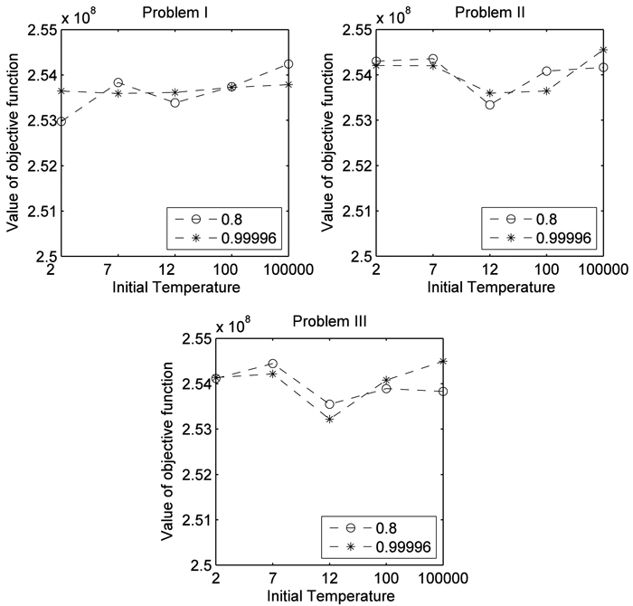
Fig. 4. Comparison of cooling scheduling (0.8 and 0.99996) and initial temperature (2, 7, 12, 100, 100000) for each problem formulation for the instance 1000 stands. Problem I encompassed the use of even-flow of harvest constraints, Problem II further included the use of ending volume inventory and carbon stock level constraints. Problem III was an extension of previous models and further included adjacency constraints.
| Table 1. Configuration of parameters (initial temperature T0, cooling schedule ζ ) for the Instance of 1000 stands. Problem I encompassed the use of even-flow of harvest constraints, Problem II further included the use of ending volume inventory and carbon stock level constraints. Problem III was an extension of previous models and further included adjacency constraints. | |||||||
| Model | Average objective | Best objective | Worst objective | Average time[s] | GAP1 1 [%] | GAP2 2 [%] | Best parameters |
| Problem I | 253654092.6 | 254242073 | 252974250 | 11560 | 0.2313 | 0.499 | T0 = 100000, ζ = 0.8 |
| Problem II | 254044417.2 | 254553811 | 253337282 | 13913 | 0.2 | 0.478 | T0 = 100000, ζ = 0.99996 |
| Problem III | 253998184.9 | 254495562 | 253219220 | 20134 | 0.1954 | 0.502 | T0 = 100000, ζ = 0.99996 |
| 1 GAP1 refers to the relative gap between the best and the average value. | |||||||
| 2 GAP2 refers to the relative gap between the best objective value found and the worst value achieved by SA. | |||||||
3.1.2 Experiment II
Opposite to experiment I, results show that for the problem solved (Problem III) and regardless of initial temperature and cooling schedule, when selecting a small number of treatment schedules available per stand (up to 15) changing the treatment schedule in two stands in each iteration (two-opt moves) implementation of the SA achieved better solutions that one- and three-opt moves (Fig. 5).
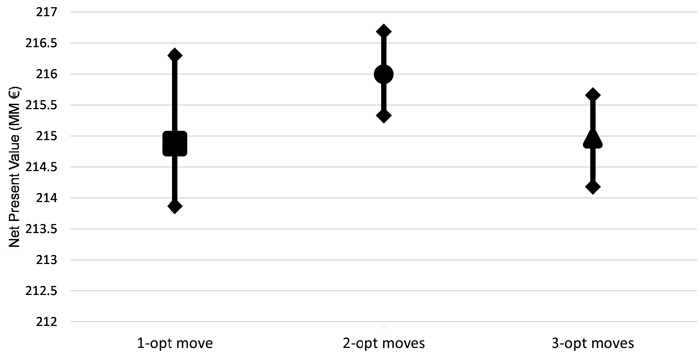
Fig. 5. Performance of the different implementations of Simulated Annealing (SA) (one, two and three-opt moves) for problem formulation III and for the instance of 1000 stands for different combinations of initial temperature and cooling schedule. Problem III corresponded to the maximization of net returns using even-flow of harvest constraints, ending volume inventory and carbon stock level constraints and adjacency constraints.
3.2 Comparison of experimental results achieved by SA and CPLEX
Results showed that problem instances of smaller size and with lower number of constraints for experiment I were easily resolved under the exact optimization methods, while for the large and very constrained problems SA algorithm implementation performed better than exact methods in terms of computational time (Table 2). In fact, for instances between 250 and 1000 stands for problems I and II, CPLEX performed better than SA. For example, for the 250 and 500 stands instances for both problems I and II, CPLEX found the optimum less than 9 minutes, while SA procedure needed 300000 iterations (around 30 minutes) to find a solution within a satisfying gap (Table 2).
| Table 2. Comparison of performance of exact (CPLEX) and heuristic (Simulated Annealing (SA)) methods. | ||||||||
| Stands | Problem | CPLEX | SA | Statistics | ||||
| Best objective | Time[s] | Gap[%]3 | Best objective | Average time[s] | Saved time[%] | Relative gap[%]4 | ||
| 100 | I | 19385252 | 6591 | 3.78 | 18208598 | 784 | 88 | 6.07 |
| 100 | II | 18787533 | 24348 | 6.93 | 18247907 | 1039 | 96 | 2.87 |
| 100 | III | 19987548 | 32813 | 0.51 | 18244260 | 1523 | 95 | 8.72 |
| 250 | I | 49576379 | 80 | 0.85 | 47641286 | 2248 | –2710 | 3.90 |
| 250 | II | 49705423 | 148 | 0.58 | 47762817 | 2775 | –1775 | 3.91 |
| 250 | III | 49535258 | 10890 | 0.92 | 47787089 | 4212 | 61 | 3.53 |
| 500 | I | 110140532 | 405 | 0.14 | 107751035 | 4967 | –1126 | 2.17 |
| 500 | II | 109921875 | 523 | 0.33 | 107789228 | 6416 | –1127 | 1.94 |
| 500 | III | 110059776 | 13460 | 0.20 | 107729193 | 9448 | 30 | 2.12 |
| 1000 | I | 261614671 | 8459 | 0.01 | 254242073 | 11560 | –37 | 2.82 |
| 1000 | II | 261604515 | 34076 | 0.01 | 254553811 | 13913 | 59 | 2.70 |
| 1000 | III | - | - | - | 254495562 | 20134 | n.a. | n.a. |
| 3 The column “Gap” refers to the default gap calculation in CPLEX and stands for the relative difference between the highest objective value and the lowest upper bound that is found during optimization process [%]. | ||||||||
| 4 The column “Relative gap” refers to the relative percentage difference between the CPLEX and SA solutions. | ||||||||
It is also important to note that although the instance size tended to increase the solution time involved, the smallest instance (i.e. using only 100 stands) was extremely time consuming in CPLEX. Although this instance can be considered as a small problem, it was a combinatorial problem very hard to solve due to the limited possibility of feasible combinations to meet the demand and flow constraints compared to instances that had a larger number of stands. Although SA overcomes this problem and finds solution in reasonable time, the result were disappointing due to a big relative gap compared to the optimal solution found in CPLEX.
Adding adjacency constraints to all instances (Problem III) increased significantly solution time in both CPLEX and SA regardless of the instances analyzed. These constraints increased the complexity of the problem and the differences between CPLEX and SA. The results show that SA obtains satisfying solutions in much shorter computing time than CPLEX. Moreover, CPLEX could not handle the adjacency constraints in large instances (e.g. instance of 1000 stands) and got out of memory. Defining adjacency constraints as lazy constraints in CPLEX did not show any improvement and in the large instances the solution was not found either. Further, the solutions obtained SA were satisfactory near-optimal with a very reasonable computation time.
4 Discussion and conclusion
In this paper we compared the performance of different implementations of a well-known heuristic technique (i.e. Simulated Annealing) when applied to a harvest scheduling problem. Similarly to the work presented by Garcia-Gonzalo et al. (2012) we implemented SA with up to three decision choice moves (one to three-opt moves). However, in addition to using the forest management problem including even-flow of harvests constraints we added adjacency constraints and a large number of candidate management schedules which largely complicates the combinatorial problem. Further, as the values of heuristic parameters are problem-specific (Borges et al. 2002) this research was influential to assess the best approach to implement SA over a wider range of forest planning problems.
Different instances of each problem were solved to analyze the impact of the size of the problem in the solution techniques. We further analyze the quality of outcomes by comparing SA solutions with the exact method performed in CPLEX. The decision variables used in this article were which treatment schedule to apply in each stand. Each treatment schedule consisted of a calendar of operations to be applied in the stand during the whole planning horizon. Since we wanted to track not only the amount of resource produced by stands over the planning horizon but also the spatial distribution of stand treatment programs we needed to ensure the integrity of the stands (i.e. stands cannot be divided). This means that a very large volume of information needed to be processed and tracked and that the size of the combinatorial problem became very large (Bettinger et al. 1999; Weintraub and Murray 2006). In order to check the sensitivity of the optimal number of decision choice moves to the number of treatment schedules available we performed two experiments: i) a large planning problem using a large set of treatment schedules available for each stand (i.e. up to 278) and ii) a smaller planning problem using reduced number of treatment schedules (i.e. up to 15).
For the problems under study, the instances of smaller size and with lower number of constraints were easily solved using exact optimization methods, while for the instances with big problems and/or very complex to solve SA algorithm performed better than the exact method. In fact for large problems with spatial concerns and/or with extremely high number of decision choices the commercial MIP solver consumed much larger computational time than SA or it was unable to solve them. Thus, for these large and constrained ARM problems we propose the use of an advanced heuristic technique instead of exact method. This pattern has been already stated by other authors (e.g. Zhu et al. 2007) who affirmed that for ARM problems and depending on the size of the instance the resulting solution solving process can easily consume the memory of a computer or the software used concluding that in these cases relying on exact optimization methods as a solution approach may not be the best option.
In our results, when analyzing what is the optimal number of changes (from one-opt to three-opt moves), the results were sensitive to the number of treatment schedules available. For a very large number of choices available one-opt move implementation was better than two or three-opt moves for any combination of initial temperature and cooling schedule. This is contrary to other results found by other authors (Bettinger et al. 1999; Heinonen and Pukkala 2004). However, they used considerably smaller number of alternative treatment schedules per management unit and their problem had significantly less decision choices. In fact, in order to test this hypothesis we run the same problem instances but reducing the number of possible management schedules to 15 (experiment II). In this test we also found that two-opt moves was better than one-opt move. Additionally we also found that three-opt moves provided inferior solutions than two and one-opt move. Since the use of one-opt move was the best option we tested if intensifying the search by using two-opt moves every a certain number of iterations would improve the results. One test was to intensify the search by using one two-opt moves every one hundred iterations, the second test was to use ten iterations with two-opt moves every hundred iterations. None of these tests improved the solutions found by using only one-opt move. Thus, we conclude that for very large problems with a large number of decision choices one-opt move is preferable.
The parameter of initial temperature is related to the number of iterations and we have showed that for a very large scale problem the search procedure requires a bigger number of iterations to achieve better solution. The impact of cooling schedule parameters was negligible.
With these results we conclude that in Simulated Annealing algorithm the number of possible treatment schedules available for each stand has an impact on the optimal configuration of opt-moves to use. When using a large set of treatment schedules available for each stand using one-opt move is preferable than two-opt moves regardless of the size of the forest (i.e. instance). If the number of decision choices per management unit is reduced then two-opt moves are preferable. On the other hand, for small problem formulations with small number of decision choices exact optimization methods provide better solutions in a reasonable time. On the contrary when large and very complex problems are to be solved and when the number of decision choices per management unit is large SA performs considerably better than CPLEX.
Acknowledgements
This research was partially supported by the projects PTDC/AGR-FOR/4526/2012 Models and Decision Support Systems for Addressing Risk and Uncertainty in Forest Planning (SADRI), funded by the Portuguese Foundation for Science and Technology (FCT - Fundação para a Ciência e a Tecnologia). It has received funding from the European Union’s Seventh Programme for research, technological development and demonstration under grant agreements: i) nr 282887 INTEGRAL (Future-oriented integrated management of European forest landscapes) and ii) nr PIRSES-GA-2010-269257 (ForEAdapt, FP7-PEOPLE-2010-IRSES).
References
Aarts E., Lenstra J.K. (eds.). (1997). Local search in combinatorial optimization. Princetwon University Press. Wiley, New York.
Alfa A.S., Heragu S.S., Chen M. (1991). A 3-OPT based simulated annealing algorithm for vehicle routing problems. Computers & Industrial Engineering 21(1–4): 635–639. http://dx.doi.org/10.1016/0360-8352(91)90165-3.
Bertomeu M., Romero C. (2001). Managing forest biodiversity: a zero-one goal programming approach. Agricultural Systems 68(3): 197–213. http://dx.doi.org/10.1016/S0308-521X(01)00007-5.
Bettinger P., Kim Y.H. (2008). Spatial optimisation - computational methods. In: Gadow K., Pukkala T. (eds.). Designing green landscapes. Vol. 15 of the book series Managing Forest Ecosystems, Springer, Dordrecht. p. 107–136. http://dx.doi.org/10.1007/978-1-4020-6759-4_5.
Bettinger P., Boston K., Sessions J. (1999). Intensifying a heuristic forest harvest scheduling search procedure with 2-opt decision choices. Canadian Journal of Forest Research 29: 1784–1792. http://dx.doi.org/10.1139/x99-160.
Bettinger P., Graetz D., Boston K., Sessions J., Chung W. (2002). Eight heuristic planning techniques applied to three increasingly difficult wildlife planning problems. Silva Fennica 36(2): 561–584. http://dx.doi.org/10.14214/sf.545.
Bettinger P., Sessions J., Boston K. (2009). A review of the status and use of validation procedures for heuristics used in forest planning. Mathematical and Computational Forestry & Natural-Resource Sciences (MCFNS) 1(1): 26–37.
Borges J.G., Hoganson H.M. (2000). Structuring a landscape by forestland classification and harvest scheduling spatial constraints. Forest Ecology and Management 130: 269–275. http://dx.doi.org/10.1016/S0378-1127(99)00180-2.
Borges J.G., Hoganson H.M., Falcão A.O. (2002). Heuristic in multi-objective forest planning. In: Pukkala T. (ed.). Multi-objective forest planning. Kluwer Academic, Dordrecht. p. 119–151. http://dx.doi.org/10.1007/978-94-015-9906-1_6.
Borges P., Eid T., Bergseng E. (2014a). Applying simulated annealing using different methods for the neighborhood search in forest planning problems. European Journal of Operational Research 233(3): 700–710. http://dx.doi.org/10.1016/j.ejor.2013.08.039.
Borges P., Bergseng E., Eid T. (2014b). Adjacency constraints in forestry – a simulated annealing approach comparing different candidate solution generators. Mathematical and Computational Forestry & Natural-Resource Sciences 6(1): 11–25.
Constantino M., Martins I., Borges J.G. (2008). A new mixed-integer programming model for harvest scheduling subject to maximum area restrictions. Operations Research 56: 543–551. http://dx.doi.org/10.1287/opre.1070.0472.
Falcão A.O., Borges J.G. (2002). Combining random and systematic search heuristic procedures for solving spatially constrained forest management scheduling models. Forest Science 48(3): 608–621.
Falcão A.O., Borges J.G. (2005). Designing decision support tools for Mediterranean forest ecosystem management: a case study in Portugal. Annals of Forest Science 62: 751–760. http://dx.doi.org/10.1051/forest:2005061.
Garcia-Gonzalo J., Borges J.G., Hilebrand W., Palma J.H.N. (2012). Comparison of effectiveness of different implementations of a heuristic forest harvest scheduling search procedure with different number of decision choices simultaneously changed per move. Lectures Notes in Management Science 4: 179–183.
Garcia-Gonzalo J., Borges J.G., Palma J.H.N., Zubizarreta - Gerendiain A. (2014). A decision support system for management planning of eucalyptus plantations facing climate change. Annals of Forest Science 71: 187–199. http://dx.doi.org/10.1007/s13595-013-0337-1.
Ghaffari-Nasab N., Jabalameli M. S, Saboury A. (2013). Multi-objective capacitated location-routing problem: modelling and a simulated annealing heuristic. International Journal of Services and Operations Management 15(2): 140–156. http://dx.doi.org/10.1504/IJSOM.2013.053642.
Goycoolea M., Murray A.T., Barahona F., Epstein R., Weintraub A. (2005). Harvest scheduling subject to maximum area restrictions: exploring exact approaches. Operations Research 53(3): 490–500. http://dx.doi.org/10.1287/opre.1040.0169.
Goycoolea M., Murray A.T., Vielma J.P., Weintraub A. (2009). Evaluating approaches for solving the area restriction model in harvest scheduling. Forest Science 55(2): 149–165.
Heinonen T., Pukkala T. (2004). A comparison of one- and two-compartment neighbourhoods in heuristic search with spatial forest management goals. Silva Fennica 38(3): 319–332. http://dx.doi.org/10.14214/sf.419.
Johnson K.N., Scheurmann H.L. (1977). Techniques for prescribing optimal timber harvest and investment under different objectives - discussion and synthesis. Forest Science Monograph 18.
Kirkpatrick S., Gelatt C.D., Vecchi M.P. (1983). Optimization by simulated annealing. Science 220(4598): 671–680.
Lockwood C., Moore T. (1993). Harvest scheduling with spatial constraints: a simulated annealing approach. Canadian Journal of Forest Research 23(3): 468–478. http://dx.doi.org/10.1139/x93-065.
McDill M.E., Braze J. (2001). Using branch and bound algorithm to solve forest planning problems with adjacency constraints. Forest Science 47(3): 403–418.
McDill M.E., Rebain S.A., Braze J. (2002). Harvest scheduling with area-based adjacency constraints. Forest Science 48(4): 631–642.
Metropolis N., Rosenbluth A.W., Rosenbluth M.N., Teller A.H., Teller E. (1953). Equation of state calculation by fast computing machines. Journal of Chemical Physics 21: 1087–1092. http://dx.doi.org/10.1063/1.1699114.
Murray A.T. (1999). Spatial restrictions in harvest scheduling. Forest Science 45(1): 45–52.
Murray A.T., Weintraub A. (2002). Scale and unit specification influences in harvest scheduling with maximum area restrictions. Forest Science 48(4): 779–789.
Nelson J., Brodie J.B. (1990). Comparison of a random search algorithm and mixed integer programming for solving area-based forest plans. Canadian Journal of Forest Research 20: 934–942. http://dx.doi.org/10.1139/x90-126.
Pham D.T., Karaboga D. (2000). Intelligent optimisation techniques: genetic algorithms, tabu search, simulated annealing and neural networks. Springer-Verlag, London. 302 p.
Pukkala T., Heinonen T. (2006). Optimizing heuristic search in forest planning. Nonlinear Analysis: Real World Applications 7: 1284–1297. http://dx.doi.org/10.1016/j.nonrwa.2005.11.011.
Pukkala T., Kurttila M. (2005). Examining the performance of six heuristic optimisation techniques in different forest planning problems. Silva Fennica 39(1): 67–80. http://dx.doi.org/10.14214/sf.396.
Reeves C.R. (ed.). (1993). Modern heuristic techniques for combinatorial problems. John Wiley & Sons, Inc. 320 p.
Snyder S., Revelle C. (1996). Temporal and spatial harvesting of irregular systems of parcels. Canadian Journal of Forest Research 26: 1079–1088. http://dx.doi.org/10.1139/x26-119.
Tóth S.F., McDill M.E., Könnyü N., George S. (2013). Testing the use of lazy constraints in solving area-based adjacency formulations of harvest scheduling models. Forest Science 59(2): 157–176. http://dx.doi.org/10.5849/forsci.11-040.
Weintraub A., Murray A.T. (2006). Review of combinatorial problems induced by spatial forest harvesting planning. Discrete Applied Mathematics 154(5): 867–879. http://dx.doi.org/10.1016/j.dam.2005.05.025.
Zhu J., Bettinger P., Li R. (2007). Additional insight into the performance of a new heuristic for solving spatially constrained forest planning problems. Silva Fennica 41(4): 687–698. http://dx.doi.org/10.14214/sf.276.
Total of 37 references
