Paulo Borges  ,
Even Bergseng,
Tron Eid,
Terje Gobakken
,
Even Bergseng,
Tron Eid,
Terje Gobakken
Impact of maximum opening area constraints on profitability and biomass availability in forestry – a large, real world case
Borges P., Bergseng E., Eid T., Gobakken T. (2015). Impact of maximum opening area constraints on profitability and biomass availability in forestry – a large, real world case. Silva Fennica vol. 49 no. 5 article id 1347. https://doi.org/10.14214/sf.1347
Highlights
- We solved a large and real world near city forestry problem
- The inclusion of maximum open area constraints caused 7.0% loss in NPV
- Solution value at maximum deviated 0.01% from the true optimum value
- The annual energy supply of 20–30 GWh estimated from harvest residues could provide a small, but stable supply of energy to the municipality.
Abstract
The nature areas surrounding the capital of Norway (Oslomarka), comprising 1 700 km2 of forest land, are the recreational home turf for a population of 1.2 mill. people. These areas are highly valuable, not only for recreational purposes and biodiversity, but also for commercial activities. To assess the impacts of the challenges that Oslo municipality forest face in their management, we developed four optimization problems with different levels of management constraints. The constraints consider control of harvest level, guarantee of minimum old-growth forest area and maximum open area after final harvest. For the latter, to date, no appropriate analyses quantifying the impact of such a constraint on economy and biomass production have been carried out in Norway. The problem solved is large due to both the number of stands and number of treatment schedules. However, the model applied demonstrated its relevance for solving large problems involving maximum opening areas. The inclusion of maximum open area constraints caused 7.0% loss in NPV compared to the business as usual case with controlled harvest volume and minimum old-growth area. The estimated supply of 20-30 GWh annual energy from harvest residues could provide a small, but stable supply of energy to the municipality.
Keywords
bioenergy;
forest management planning;
mixed integer programming;
area restriction model;
green-up
-
Borges,
Department of Ecology and Natural Resource Management, Norwegian University of Life Sciences, P.O. Box 5003, 1432 Aas, Norway
E-mail
paulo.borges@nmbu.no
- Bergseng, Department of Ecology and Natural Resource Management, Norwegian University of Life Sciences, P.O. Box 5003, 1432 Aas, Norway E-mail even.bergseng@nmbu.no
- Eid, Department of Ecology and Natural Resource Management, Norwegian University of Life Sciences, P.O. Box 5003, 1432 Aas, Norway E-mail tron.eid@nmbu.no
- Gobakken, Department of Ecology and Natural Resource Management, Norwegian University of Life Sciences, P.O. Box 5003, 1432 Aas, Norway E-mail terje.gobakken@nmbu.no
Received 7 April 2015 Accepted 10 July 2015 Published 1 September 2015
Views 194864
Available at https://doi.org/10.14214/sf.1347 | Download PDF

Introduction
Forests provide multiple commodities such as ecosystem services, recreational values and economic gains. Decision-making in forest management, which includes an increasing number of commodities, many decision levels as well as spatial and temporal aspects, is a highly challenging task. Modelling such management is complex, analyses are time consuming and resource demanding, and require sophisticated and efficient solution methods to deal with the large amounts of data involved. The forest areas surrounding the capital of Norway (Oslomarka) are an example of a forest area where management and decision-making take place in a highly complex environment.
Oslomarka, comprising 1700 km2 of forest land located in five different counties (Oslo, Akershus, Buskerud, Oppland and Østfold), is the recreational home for a population of 1.2 mill. people (Ministry of Environment 2013). These areas are highly valuable, not only for recreational purposes and biodiversity, but also for commercial activities related to forestry and other industries. For a forest located close to a large city, potential energy production might be of more interest than the output in terms of volume of sawn wood and pulpwood. Energy from harvest residues could provide a small, but stable supply of energy to the municipalities. Activities relating to nature areas in Oslo and nearby municipalities are regulated by legislation, the Marka law (Act No. 35 of 5th June 2009). The major part of the area (70%) is privately owned, while the remaining areas are managed by municipalities or through commons. Most of the approximately 2 000 forest properties within Oslomarka are very small, but the largest property is a privately owned industrial forest (430 km2) and the second largest is the Oslo municipality forest (about 160 km2). There are obvious user conflicts in Oslomarka between a large population using the forest land for recreational purposes and sporting activities, a strong environmental lobby that wants to preserve as large areas as possible for biodiversity purposes and the forest owners with their commercial interests.
In addition to the Marka law, commercial forestry activities in Oslomarka are influenced by the Forestry Act (Act No. 31 of 27th May 2005). All forestry activities in Oslomarka are, like most of Norway, under the present PEFC certification regime (Norsk Skogsertifisering 2013), which is based on the standard “Living Forests: Standard for sustainable forest management in Norway” (Living Forest 2010). Local preferences are also reflected in the management. For example, the multi-purpose forest management plan for the part of Oslomarka belonging to Oslo municipality clearly states that “economic considerations are inferior to recreational and biological considerations” (Oslo Municipality 2007). Despite the environmental emphasis, roundwood is harvested and provides income for the municipality. Often referred to as the “green city” due to the large share of renewable energy in Oslo, with the municipality itself producing energy at two waste disposal plants, the forest is also a potential source of renewable energy.
The prevalent legislation and certification regime obviously have consequences for forest management and the subsequent possible range of silvicultural treatments, and accordingly also for profitability and quantities of timber and biomass to be harvested. In Norway, many studies have tried to quantify some of these consequences. As a scientific foundation for developing the “Living Forests standards” more than a decade ago, several comprehensive analyses quantified consequences of environmentally oriented constraints at national, regional and property level (Hoen et al. 1998, 2001; Eid et al. 2001, 2002). Later also Ask et al. (2005) and Bergseng et al. (2012, 2013) performed similar analyses focusing on consequences of environmentally oriented constraints on forest management.
The tool applied for all these analyses consists of a growth simulator (GAYA) and an optimization (J) tool controlled from a geographical information system (SGIS). First, GAYA simulates numerous treatment schedules for each stand (Hoen and Eid 1990; Hoen and Gobakken 1997; Gobakken 2003) and then the management problem is solved at forest level by linear programming (LP) using the J algorithm (Lappi 1992, 2003). Connecting GAYA, J and SGIS makes each stand an identifiable polygon with respect to forest characteristics. The environmentally oriented constraints considered in these studies have included for example maximum sustainable harvest levels (or maximum variations in harvest level over time), maintaining minimum proportions of old-growth forest, prolonged rotation cycles, retention trees, selective cutting in buffer zones related to key biotopes and water bodies (rivers and lakes). In the most comprehensive of these studies (Bergseng et al. 2012), the impacts on both economy and biodiversity were analysed based on data from Ski municipality forest with a management reflecting the local preferences as well as the current Norwegian forest certification system. Economic impacts were expressed as changes in net present value (NPV) and harvest level, while impacts on forest structure were expressed by variables such as old-growth proportions, growing stock, number of retention trees, size of buffer zones and amount of dead wood.
All the environmentally oriented constraints considered in these studies have been incorporated by means of simulations and linear programming. In the case of Oslomarka, however, there is an additional modelling challenge related to management as local regulations (Act No. 35 of 5th June 2009) defines that the connected open area after final harvests (clear cutting and seed tree cutting) should not exceed 3 ha. Although not specified in the regulations, this also means that adjacent areas cannot be harvested before the areas have been regenerated and trees have reached a height, which “visually can be considered as a forest”. The motivation for including such constraints in forest management may be to reduce the effects of clear cutting on forest fragmentation and ecological processes, to disperse the potential impact on water quality from harvesting or to develop a forest with a variety of different age classes that favour high species richness. However, since Oslomarka is used by so many people, recreational and aesthetic aspects have been a main motivation (Gundersen et al. 2015).
Controlling harvested volume over time is one of the most used requirements in forest planning (Shan et al. 2009). Both in Norway and internationally there has been quite a lot of development to deal with such management. The common approach is a non-declining or even flow of harvested volume (e.g. Daust and Nelson 1993; McDill and Braze 2000; Hoen et al. 2001; Caro et al. 2003). More flexible approaches have also been used, such as allowing variations in the harvested volume, i.e. ensuring that it does not vary more than a certain percentage between consecutive planning periods (e.g. Falcão and Borges 2002; Rebain and McDill 2003; Crowe and Nelson 2005; Constantino et al. 2008; Borges et al. 2014ab) or by letting the model decide the optimal levels of harvest (Martins et al. 2014). Furthermore, requirements for maintaining minimum proportions of old-growth forest have frequently been addressed. This type of management can be implemented by simply requiring a percentage of the total area to be old-growth forest in each planning period or it may be extended by specifying the amount of area in old-growth for each site quality class present in the forest area (e.g. Eid et al. 2001, 2002).
The previous requirements are affected by the spatial structure in the landscape, i.e. the relative arrangement of patches or the relative arrangement of harvest areas. In general, there are two different approaches when including spatial considerations in forest planning: the exogenous approach and the endogenous approach. When the exogenous approach is used, no spatial information is included in the optimization algorithm. Instead, the optimization process uses predetermined spatial constraints (e.g. Bergseng et al. 2012). In the endogenous approach, the optimization algorithms include spatial information and the optimization process determines the spatial arrangement of features such as harvested areas or old forest stands (e.g. Murray 1999; Öhman 2000). One advantage of the latter approach is that this approach can evaluate a very large number of spatial arrangements and allow trade-off analyses between different objectives. However, if the endogenous approach is used, effective constraint structures and efficient optimization models must be developed to control the impacts of management activities in one area on the surrounding areas.
A spatial endogenous approach widely used in forest planning is constraining the size of final harvests to a maximum area (e.g. Thompson et al. 1973; Murray 1999; McDill and Braze 2000). This type of constraint is known as adjacency constraints in harvest scheduling and the works of Roise (1990), Nelson and Brodie (1990), Dahlin and Sallnäs (1993), Weintraub et al. (1994) and Borges et al. (1999) were pioneering approaches to model and solve problems involving these constraints. Depending on the size of stands relative to the maximum final harvest area, two approaches can be applied. The unit restriction model (URM) constraints harvest of neighbouring stands while the area restriction model (ARM) constraints the area of final harvests to a maximum area of contiguous stands (Murray 1999). The constraints that prohibits final harvest in stands before final harvested areas have been regenerated is known in forest planning as green-up constraints. The URM and ARM approaches are specific cases of green-up constraints where the green-up time (regeneration of final harvested areas) is one planning period, which coincides with the planning period when the final harvest occurs. In both URM and ARM approaches, extending the green-up time for more than one planning period lead to a more general concept known as maximum opening area (MOA) constraints, where an open area is defined either as an area finally harvested or as an area in a regeneration state (e.g. Boston and Sessions 2006). The aim is then to guarantee that MOA is not exceeded (e.g. Crowe et al. 2003; Gunn and Richards 2005; Goycoolea et al. 2005, 2009; Borges et al. 2015).
Most of the forest planning literature involving green-up constraints assume a fixed length for green-up (Shan et al. 2009). However, modelling green-up constraints with a fixed length for green-up does not reflect entirely the dynamics of forestry. The regeneration strategy (Boston et al. 2009) as well as site productivity of stands (Borges et al. 2015) have influence on the time that a stand needs to regenerate, i.e. time for trees to reach a certain height where the stand is no longer considered as an open area. By considering variable length for the green-up time, the economic impact of such constraints may be reduced (Boston et al. 2009; Borges et al. 2015).
To our knowledge, the studies of Boston et al. (2009) and Borges et al. (2015) are the only ones that have considered a variable length for green-up time. Boston et al. (2009) treated the green-up length as a decision variable and different regeneration efforts were tested. Borges et al. (2015) retrieved the green-up length for each stand from empirical data by considering tree species and site index of each stand. They also used height predicted from a growth model to formulate the MOA constraints. However, only planting was used as regeneration method. This is obviously a simplification of the real situation where natural regeneration is an important option. In Norwegian forest conditions, it is optimal to regenerate using planting only for medium and high site productivity. However, the green-up constraint will also influence the choice of regeneration because shortening the green-up will open the possibility for harvesting neighbouring stands.
The forest problems considered in both of these studies were relatively small in terms of number of stands and respective treatment schedules. Nevertheless, due to the nature of these type of problems (mixed-integer), the respective solution space and solving time can be large even for small problems. Therefore, when addressing “real” and “large” problems with a large number of stands, planning periods and regeneration options, such as in the Oslo municipality forest, it is important to demonstrate alternative problem formulations that can be solved within a reasonable amount of time. Moreover, in Norway, real case studies involving spatial endogenous approaches such as considering maximum opening area constraints in final harvests are scarce. The works from Hasle et al. (2000) and Stølevik et al. (2007) are the fewest in Norway. In both works, the authors used heuristic procedures to solve problems encompassing 700 and 1 541 forest stands.
The main objective of this study is to model and quantify the impact of maximum opening area constraints on profitability and biomass availability for Oslo municipality forest. We combine the ideas and experience from Boston et al. (2009) and Borges et al. (2015) in a large, real world case where the green-up constraints reflect the effects of different regeneration options (planting and natural regeneration), regenerated tree species and site productivity of each stand. Additionally, we explore management options and constraints related to controlled harvest volume and minimum old-growth forest areas, and their effects. In all analyses, we use forest inventory data covering the entire Oslo municipality forest.
2 Material and methods
2.1 Site and management descriptions of Oslo municipality forest
The basis for our analyses is a forest inventory from 2010 carried out by the inventory company Foran Norway AS. According to this, the Oslo municipality forest property covers a total area of 15 538 ha, of which 12 508 ha is forest area and 12 084 ha is productive forest area. The tree species distribution (based on volume) are spruce (58%), pine (31%) and deciduous (11%), generating a total volume of 1.84 million m3. The productive forest areas distributed over ages classes and site index classes are shown in Table 1. Site index is presented according to the H40-system, i.e. dominant height in meters at breast height age 40 years (Tveite 1977; Braastad 1980).
| Table 1. Relative distribution of the productive forest area (%) distributed over age class (years) and site index (H40 - m). | ||||||||
| Site index | ||||||||
| Age class | < 7.5 | [7.5, 9.5[ | [9.5, 12.5[ | [12.5, 15.5[ | [15.5, 18.5[ | [18.5, 21.5[ | ≥ 21.5 | Total |
| 0–10 | 0.02 | 0.02 | 0.3 | 0.3 | 0.2 | 0.04 | 0.9 | |
| 11–20 | 0.1 | 0.2 | 0.1 | 1.1 | 1.0 | 0.4 | 0.02 | 2.9 |
| 21–30 | 0.02 | 0.5 | 0.2 | 3.4 | 3.9 | 0.7 | 0.02 | 8.7 |
| 31–40 | 0.01 | 0.3 | 0.2 | 3.5 | 1.9 | 0.7 | 0.1 | 6.8 |
| 41–50 | 0.1 | 1.2 | 0.3 | 5.0 | 4.6 | 1.2 | 0.3 | 12.6 |
| 51–60 | 0.3 | 1.1 | 0.3 | 6.8 | 4.2 | 1.6 | 0.7 | 15.1 |
| 61–70 | 0.1 | 0.7 | 0.1 | 4.0 | 3.0 | 1.4 | 0.2 | 9.5 |
| 71–80 | 0.3 | 0.9 | 0.4 | 2.1 | 1.7 | 0.6 | 0.0 | 6.1 |
| 81–90 | 0.8 | 1.3 | 0.2 | 2.3 | 1.5 | 0.2 | 0.01 | 6.3 |
| 91–100 | 0.4 | 1.2 | 0.3 | 1.8 | 1.2 | 0.1 | 5.1 | |
| 101–110 | 1.1 | 2.4 | 0.5 | 2.4 | 1.0 | 0.1 | 7.5 | |
| 111–120 | 0.7 | 1.2 | 0.5 | 1.3 | 0.7 | 0.1 | 4.6 | |
| > = 121 | 5.1 | 3.7 | 1.4 | 2.9 | 0.6 | 0.0 | 13.8 | |
| Total | 9.2 | 14.7 | 4.7 | 36.8 | 25.8 | 7.5 | 1.4 | 100.0 |
According to the forest inventory, the productive forest area is divided into 7 081 stands. Due to the constraints on maximum opening areas, we have split all stands larger than 3 ha randomly. The only requirement is that after the splitting, the resulting stands should at least be greater than 100 m2. This area is the minimum area that the growth simulator GAYA accepts for simulation of treatment schedules. After splitting, the total number of stands is thus 8 874, the average stand size is 1.41 ha with minimum 0.01 ha and maximum 2.99 ha. The distribution of the stands over different size classes is shown in Table 2.
| Table 2. Distribution of the stands over size classes. | ||||||||||||
| Size class (ha) | 0.00– 0.25 | 0.25– 0.50 | 0.50– 0.75 | 0.75– 1.00 | 1.00– 1.25 | 1.25– 1.50 | 1.50– 1.75 | 1.75– 2.00 | 2.00– 2.25 | 2.25– 2.50 | 2.50– 2.75 | 2.75– 3.00 |
| No. of stands | 404 | 858 | 953 | 826 | 853 | 893 | 972 | 912 | 762 | 598 | 468 | 375 |
The management of the Oslo municipality forest is based on a multi-purpose plan for the period 2007–2015 (Oslo Municipality 2007). The plan is made in cooperation with a stakeholder group consisting of representatives of different user groups like recreationists and nature conservationists. The plan clearly states targets and guidelines for management: conserving natural and cultural aspects is of paramount importance, including enhancement of activities like recreation, skiing, fishing and cycling.
Management has changed dramatically over the years, with a decrease in harvest volumes from 25 000 m3 to 8 500 m3 annually over the past 15 years. This is due to the need for increasing old-growth area and more focus on recreational values. The management plan states that from 2010 the harvest level may be increased to 13 500 m3 per year from 2010. In the medium long term, 15 to 20 years from now, annual harvest of 20 000 m3 is considered realistic.
2.2 Analysis
2.2.1 Simulations
The growth simulator GAYA (Hoen and Eid 1990; Hoen and Gobakken 1997; Gobakken 2003) was applied to generate treatment schedules. The simulator takes as input data from the stands (age, site index, number of trees and basal area per ha, basal area mean diameter, dominant height, mean height by basal, etc.) and a set of rules which define how and when forest treatments may be applied. The output provides detailed information on common forest state variables (e.g. standing volumes, age) as well as treatments (e.g. harvested volumes) and corresponding economic values (incomes and costs) for each treatment schedule and for all planning periods. In addition, the NPV based on an infinite planning horizon, is provided for each treatment schedule. We applied a 3% real rate of return.
In the present study, we allowed the following treatments; natural regeneration and planting, pre-commercial thinning, conventional thinning and the two final harvest options clear cutting and seed tree cutting. Natural regeneration can also occur after a clear cutting. In seed tree cutting, a certain number of seed trees are left in forest at the time of final harvest. The seed trees are removed a certain number of years later depending on site index. This means that not only final harvests contribute to the harvested volume in a planning period but also seed tree removal and conventional thinning. Additionally, the different regeneration options have different economic efforts and have impact on the height development of a stand. Simulations were performed for ten 5-year planning periods (50 years planning horizon). The total number of treatment schedules generated was 319 033, i.e. an average of about 36 per stand, which produces a solution space of about 368874 solutions.
Compared to most previous works (see e.g. Murray and Church 1996; McDill and Braze 2000; Richards and Gunn 2000; Bettinger et al. 2002; Boston and Bettinger 2006; Tóth et al. 2013), where clear cutting is the only final harvest option, our approach include two final harvest options. It is also important to note that the two final harvest options have different implications for the regeneration costs and regeneration lag (time from harvest to establishment of new forest). The lag for a stand to regenerate after seed tree cutting may be 10–15 years depending on site index and tree species while planting takes place immediately after clear cutting. However, in seed tree cutting there is only a small or no direct regeneration costs while for planting both plant purchase costs and labour costs are included.
Forest fuel for energy purposes, i.e. harvest residues from roundwood harvests, are quantified using biomass expansion factors from Lehtonen et al. (2004). Following the procedures of Rørstad et al. (2010), we arrive at an estimate for retrievable amount of harvest residues. Cost of residue extraction (EUR ton–1) is estimated at stand level according to Nurmi (2007) and Rørstad et al. (2010), where estimates of productivity (ton h–1) are combined with machine costs (EUR h–1). To convert biomass into energy, we assume a fixed lower heating value equal to 5320 kWh ton–1 dead matter (d.m.). (19.2 GJ ton–1 d.m.) and 30% moisture content (of green weight). This means that the effective heating value delivered end user, i.e. exclusive of energy use efficiency, is 5029 kWh ton–1 d.m. (18.1 GJ ton–1 d.m.). By multiplying supply by this factor we get the supply in kWh (GJ).
2.2.2 General model
The general model maximizes NPV. Only one treatment schedule was allowed within a stand. The general model also account for the harvested volume and the total area of old-growth forest in each planning period. Thus, the mathematical formulation was as follows:
where,
N is the set of stands
TSi is the set of treatment schedules within stand i
T is the set of planning periods
PAi is the productive area of stand i
Ai is the area of stand i
Oit is the set of treatment schedules of stand i that produce an old-growth forest area in planning period t
HVt is total harvested volume in planning period t
OGt is total old-growth forest area in planning period t
hvikt is harvested volume in planning period t in stand i when treated by treatment schedule k
npvik is the NPV associated with stand i when treated by treatment schedule k
The decision variables yik takes the value 1 if treatment schedule k is applied to stand i, and 0otherwise. Thus, equation (1) defines the objective function which maximizes NPV, equation (2) defines the NPV, equations (3) and (6) secures that only one treatment schedule is allowed per stand, equation (4) and (5) define the total harvested volume and the total old-growth forest area in each planning period, respectively. Finally, (6) defines the domain of the decision variables. Moreover, the set Oit (old-growth forest area) was built taking into consideration both the age and the site quality (Eid et al. 2001, 2002). Thus, a stand is considered to be an old-growth forest area if the age ≥ 78, 91, 104, 117 130, 143 and 156 years, respectively, for site index H40 ≥ 21.5 m, 18.5 m ≤ H40 < 21.5 m, 15.5 m ≤ H40 < 18.5 m, 12.5 m ≤ H40 < 15.5 m, 9.5 m ≤ H40 < 12.5 m, 7.5 m ≤ H40 < 9.5 m and H40 < 7.5 m.
2.2.3 Problems
We developed four problems to assess the impacts of the challenges that the Oslo municipality face in their forest management (Table 3). These problems are constructed by successively adding constraints one at the time. The first problem is a “non-constrained” (Nc) optimization problem. The types of constraints successively added are “controlled harvest volume” (Ch), “minimum old-growth forest area” (Og) and “maximum open area” (Oa). We obtained the solutions of the four problems by using CPLEX 12.5 in an Intel(R) Xeon(R) X5650 with 2.67GHz CPU. Maximum run time allowed was 14 400 seconds and the number of threads was set to four.
| Table 3. List of problems and the respective types of constraints added successively to the general model. | |||
| Problem | Type of constraint | ||
| Controlled harvest volume | Minimum old-growth forest area | Maximum open area | |
| 1- Non Constrained (Nc) | - | - | - |
| 2- Controlled harvest volume (Ch) | X | - | - |
| 3- Controlled harvest volume + Minimum old-growth forest area (ChOg) | X | X | - |
| 4- Controlled harvest volume + Minimum old-growth forest area + Maximum open area (ChOgOa) | X | X | X |
The four problems and their respective formulations were as follows;
Problem 1. Non-Constrained (Nc):
The non-constrained problem formulation is described by the general model. Although termed non-constrained, the general model requires that only one treatment schedule is selected for each stand. This is formulated as a constraint in the model. As no other constraints are included, the treatment schedule with the highest NPV is selected for each stand.
Problem 2. Controlled harvest volume (Ch):
For Problem 2, we follow the implementation described by Borges et al. (2015) where the harvest volume in a planning period t (HVt) is not allowed to change more than a certain percentage from the harvested volume in the previous planning period. This implementation also forces the harvest volume in period 1 to be constrained by the harvest volume in the last planning period. This prevents a unique trend (usually decreasing in old forests) in the flow of the harvested volume over the planning horizon to occur. For this problem, the following set of inequalities was added to the general model;
where inequalities (7) and (8) define the variation allowed for the harvested volume between consecutive planning periods. The values of α1 and α2 define the levels of allowed variation in harvests and were set to 0.9 and 1.1, respectively, and correspond to a 10% allowed variation.
Problem 3. Controlled harvest volume + Minimum old-growth forest area (ChOg):
This problem extends Problem 2 by also requiring a minimum percentage of old-growth forest to be present in all planning periods. Thus, in addition to the constraints defined for Problem 2, the following inequality was added to the general model;
The values of βt define the percentage of the total area in planning period t that should be in an old-growth forest state. β was set to 0.2 for each period t meaning that at least 20% of the total forest area should be old-growth forest at all times. However, because the potential maximum amount of old-growth forest in the first four planning periods is below 20% of the total forest area (2 502 ha), i.e. 916, 1 202, 1 657 and 2 055 ha respectively in periods 1, 2, 3 and 4, we only consider this constraint for ![]() . This means that old-growth forest areas should increase over time until period 5.
. This means that old-growth forest areas should increase over time until period 5.
Problem 4. Controlled harvest volume + Minimum old-growth forest area + Maximum open area (ChOgOa):
Problem 4 extends Problem 3 by adding a constraint on maximum open area. Since the simulation performed considers different final harvest options, i.e. clear cutting followed by planting or natural regeneration and seed tree cutting followed by natural regeneration, a formulation suggested by Borges et al. (2015) using tree height information (retrieved from the simulations) was applied. This approach has two advantages. First, it allows different green-up times (i.e. time from the final harvest until new trees are established and have reached a certain height) needed for the different regeneration options (planting and natural regeneration) without the need for additional decision variables (binary) to describe which regeneration option applied (see Boston et al. 2009). Second, this formulation indirectly considers the site index of the stands, i.e. the height information given by the GAYA simulator is a function of site index (Strand 1967; Tveite 1977; Braastad 1980).
Thus, the additional sets of constraints to be added to Problem 3 are as follows;

where, Zit is the set of treatment schedules of stand i producing a final harvest in planning period t, ![]() is the set of treatment schedules of stand i producing a height less or equal to µ meter in planning period t but not final harvest, Λ is the set of all minimally infeasible clusters. A minimally infeasible cluster is a set of stands with combined area greater than the MOA, and if a stand is removed from the cluster, the remaining stands in the cluster(s) will have a combined area less than or equal to the MOA (McDill et al. 2002).
is the set of treatment schedules of stand i producing a height less or equal to µ meter in planning period t but not final harvest, Λ is the set of all minimally infeasible clusters. A minimally infeasible cluster is a set of stands with combined area greater than the MOA, and if a stand is removed from the cluster, the remaining stands in the cluster(s) will have a combined area less than or equal to the MOA (McDill et al. 2002).
The decision variables zit takes the value 1 if stand i is finally harvested in planning period t, and 0otherwise. The decision variables wit takes the value 1 if stand i is less than µ meter at planning period t but not from a final harvest in the same period and 0otherwise. Also the decision variable xit takes the value 1 if stand i is in an open state (areas larger than the maximum limit of 3 ha with a tree height below the minimum requirement of 2 meters) in planning period t, and 0otherwise. There is no need to declare these variables as binary, since the formulation will naturally force them to be either zero or one (for details, see Borges et al. 2015). Equations (11) and (12) relate variables yik with variables zit and wit, respectively. Equation (13) defines the open state of a stand i in planning period t, where open state occurs due to final harvested or if tree height is below the minimum requirement. Inequality (14) defines MOA constraints, i.e. the path constraints as described by McDill et al. (2002). For each minimally infeasible cluster, it is necessary to ensure that at least one stand of the cluster is not selected to avoid forming an open area (area in open state). In the present study, MOA and µ were set to 3 ha and 2 meters, respectively.
3 Results
Net present value of Problem 1 (Non-constrained) was 67.8 mill. EUR while NPV of Problem 4 (Controlled harvest volume, minimum old-growth area and maximum open area) was 53.0 mill. EUR. The relative difference between these two problems in NPV, i.e. NPV-loss, was 21.8% (Table 4). When adding the MOA constraint to the other constraints, i.e. when comparing Problem 3 and 4, the NPV-loss was 7.0%.
| Table 4. NPV of each problem and NPV-loss between problems. | ||||
| Problem | NPV | NVP-loss between problems (%) | ||
| (mill. EUR) | 2- Ch | 3 - ChOg | 4- ChOgOa | |
| 1- Nc | 67.8 | 2.1 | 15.9 | 21.8 |
| 2- Ch | 66.4 | - | 14.2 | 20.2 |
| 3- ChOg | 57.0 | - | - | 7.0 |
| 4- ChOgOa | 53.0 | - | - | - |
Harvested volumes for the different harvest options over planning periods and problems are displayed in Fig. 1. In the non-constrained problem (Problem 1-Nc), the first-period harvest is very large compared to other periods and compared to the other problems. This is due to the large areas of present old forest (see Table 1). Harvest volumes for period 1, and in total over all period, generally decrease when more constraints are added (Nc → Ch → ChOg → ChOgOa). Furthermore, over the first four periods harvest volumes generally decrease. After that, the pattern is less clear. In Problem 1, harvest volumes fluctuate according to how much mature forest area available in the respective periods. The other problems show a similar increasing trend in harvest volumes, with an exception of Problem 4, where the harvest volume decreases slightly in the last period.
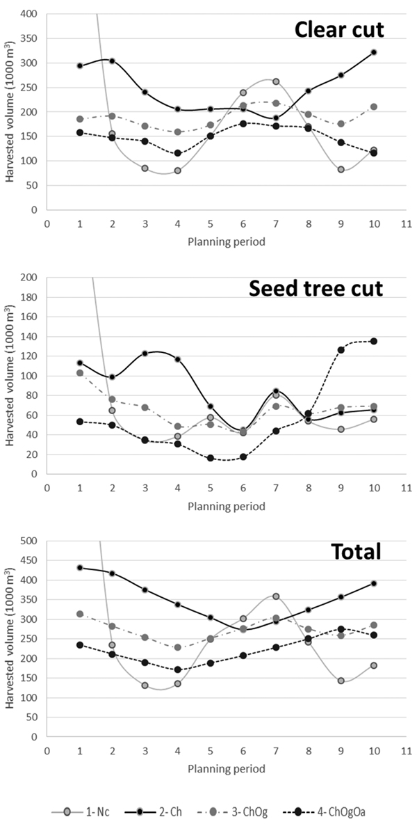
Fig. 1. Harvested volume (1000 m3) for different harvest options over planning periods and problems. First period harvested volume of Problem 1: clear cut = 741 000 m3, seed tree cut = 305 000 m3 and total = 1 071 000 m3. Problem 1. Non-Constrained (1-Nc); Problem 2. Controlled harvest volume (2-Ch); Problem 3. Controlled harvest volume + Minimum old-growth forest area (3-ChOg); Problem 4. Controlled harvest volume + Minimum old-growth forest area + Maximum open area (4-ChOgOa).
Fig. 2 shows how areas allocated to regeneration method vary over planning periods and problems. Generally the amount of regenerated areas is closely correlated to harvests (Fig. 1) resulting in decreasing areas when more constraints are added. When considering all problems, the proportions of area allocated to planting and natural regeneration are varying in the interval between 20–80% over the periods. For Problem 4, the proportions of area regenerated by planting are constantly higher than natural regeneration for the first eight planning periods. For the last two planning periods, however, more than 70% of the harvested area is regenerated naturally. For Problems 1, 2 and 3, however, no particular regeneration patterns occur over planning periods.
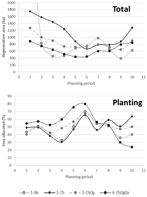
Fig. 2. Total regenerated area (ha) and regenerated area (%) allocated to planting over planning periods and problems. First period total regenerated area for Problem 1 = 4718 ha. Problem 1. Non-Constrained (1-Nc); Problem 2. Controlled harvest volume (2-Ch); Problem 3. Controlled harvest volume + Minimum old-growth forest area (3-ChOg); Problem 4. Controlled harvest volume + Minimum old-growth forest area + Maximum open area (4-ChOgOa).
The areas of old-growth increase when the requirement for old-growth areas is implemented (Problems 3 and 4) (see also Table 3). From planning period 5, the required 20% of old-growth forest is fulfilled for both problems and is held constant for the remaining periods. No accumulation of old-growth forest is observed in Problems 1 and 2. Table 5 shows the percentage of area in old-growth forest that remains as old-growth over the planning periods for Problems 3 and 4. For example, out of the 768 ha of old-growth forest present in period 1 in Problem 3, 100% still exist in period 5 before it decreases from 97% to 87% over the last five periods. Generally for both problems, almost all the existing old-growth forest from planning periods 1 to 4 also remains in period 5. From planning period 5 and onwards, at least 90% of the old-growth forest remains from one period to the next. The percentage of old-growth forest existing in planning period 5 that still exist in period 10, is 81% and 72% for Problems 3 and 4, respectively.
| Table 5. Old-growth forest areas (ha) over the planning periods, and share of old-growth forest that remain over planning periods for Problems 3 and 4. | |||||||||||
| Problems | Old-growth forest area (ha) | Planning periods | 2 | 3 | 4 | 5 | 6 | 7 | 8 | 9 | 10 |
| 3- ChOg | 768 | 1 | 100 | 100 | 100 | 100 | 97 | 93 | 93 | 89 | 87 |
| 1040 | 2 | 100 | 100 | 100 | 97 | 90 | 89 | 85 | 83 | ||
| 1487 | 3 | 100 | 100 | 96 | 88 | 87 | 84 | 83 | |||
| 1870 | 4 | 100 | 95 | 87 | 85 | 82 | 81 | ||||
| 2502 | 5 | 96 | 87 | 85 | 82 | 81 | |||||
| 2502 | 6 | 91 | 90 | 87 | 85 | ||||||
| 2502 | 7 | 99 | 95 | 94 | |||||||
| 2502 | 8 | 97 | 95 | ||||||||
| 2502 | 9 | 98 | |||||||||
| 2502 | 10 | ||||||||||
| 4- ChOgOa | 776 | 1 | 99 | 99 | 99 | 99 | 94 | 88 | 85 | 83 | 81 |
| 1048 | 2 | 100 | 100 | 100 | 94 | 83 | 80 | 77 | 76 | ||
| 1491 | 3 | 100 | 100 | 94 | 84 | 82 | 78 | 75 | |||
| 1870 | 4 | 100 | 93 | 83 | 80 | 75 | 72 | ||||
| 2502 | 5 | 94 | 84 | 80 | 75 | 72 | |||||
| 2502 | 6 | 90 | 86 | 80 | 77 | ||||||
| 2502 | 7 | 96 | 89 | 85 | |||||||
| 2502 | 8 | 92 | 88 | ||||||||
| 2502 | 9 | 95 | |||||||||
| 2502 | 10 | ||||||||||
Fig. 3 shows how the amount of areas in open state develops over periods. For Problem 4, where the open area and height requirements are implemented, there are still open areas in the first five planning periods (94, 33, 24, 24 and 8 ha, respectively) caused by already existing open areas before the simulations started. The amount of open areas from planning period 6 is zero. For the other problems, the open areas generally accumulate over the first periods, then stabilize and partly decrease again.
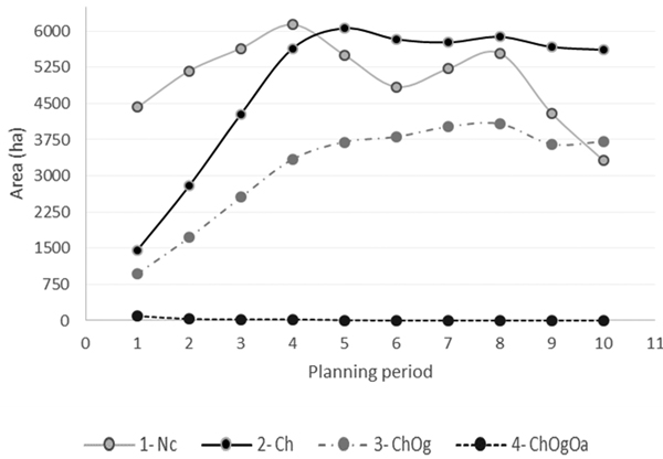
Fig. 3. Total area (ha) in open state over planning periods and problems. Problem 1. Non-Constrained (1-Nc); Problem 2. Controlled harvest volume (2-Ch); Problem 3. Controlled harvest volume + Minimum old-growth forest area (3-ChOg); Problem 4. Controlled harvest volume + Minimum old-growth forest area + Maximum open area (4-ChOgOa).
For a selected part of the municipality forest, Fig. 4 shows open state and old-growth forest areas in planning period 5 for Problems 3 and 4. For both problems, much of the old-growth forest area is the same. However, the patches of open areas are reduced considerably when introducing the MOA constraints (Problem 4).
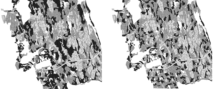
Fig. 4. Open state and old-growth forest areas for problem 3 (left) and problem 4 (right) in period 5. Old-growth forest (light grey), young forest (grey) and areas in open state (black).
The maximum energy potential for the different problems in different periods is shown in Fig. 5. The potential in period 1 for Problem 4 is 26.5 GWh. The energy potential closely follows harvest patterns (Fig. 1), and all problems with constraints on the harvest volume (2, 3 and 4), show the same general pattern with a slight decrease in the first periods and then an increase. For Problem 4, where all the constraints are implemented, the forest is able to provide 20–30 GWh annually from harvest residues over the 50-year period.
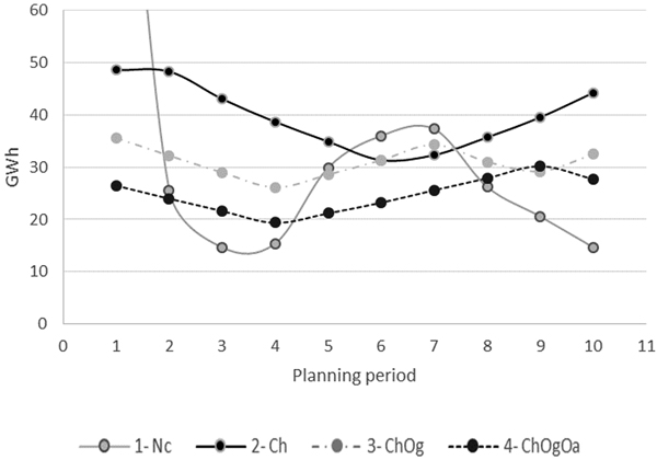
Fig. 5. Maximum energy potential from harvest residues over planning periods and problems. First period energy potential for Problem 1 = 124 GWh. Problem 1. Non-Constrained (1-Nc); Problem 2. Controlled harvest volume (2-Ch); Problem 3. Controlled harvest volume + Minimum old-growth forest area (3-ChOg); Problem 4. Controlled harvest volume + Minimum old-growth forest area + Maximum open area (4-ChOgOa).
4 Discussion
The present study models and investigates the effects of certain constraints on forest management in a large, area real world urban forest case covering the entire Oslo municipality forest. The constraints comprise a controlled level of harvest flow over time, a minimum requirement of areas with old-growth forest and a requirement of maximum open area (MOA). The constraints on maximum size of open area are statutory, and impose a series of adjacency dependencies that directly effects harvest options. The modelling of such management constraints is challenging to handle in an optimization framework, and analyses are time consuming and resource demanding, especially because our case study area is large. In this study, we combine ideas and experiences from Boston et al. (2009) and Borges et al. (2015), and mimic the management associated with this forest when solving the optimization problem. In the following, we first discuss some of the modelling challenges and then elaborate on some of the practical effects related to the management.
The initial distribution of stands with respect to size and site characteristics (see Table 2) is important when there is a requirement for MOA. Previous studies such the ones from Barret (1997) and, Borges and Hoganson (1999, 2000) have shown that the way stands are split to address MOA constraints have influence in both economic and spatial features (e.g. old growth area , types of edge). However, no specific rules regarding the way stands should be split are stated in the Marka law (Act No. 35 of 5th June 2009) and future work can be performed in this direction. The random splitting applied has increased the number of stands by 20% leading to a forest where 34% of the stands have an area lower than 1ha. This also influence the respective optimization problems since they can become difficult to solve if there are several clusters (contiguous stands) with many stands that can potentially form open areas in the same planning period. This is the case when the size of a typical stand is relatively small compared to the size of the MOA (e.g. McDill et al. 2002; Goycoolea et al. 2009). These concerns relate to the procedures that detect all the needed constraints, which are usually time demanding to compute, and to the time to solve the problem as well as the quality of the respective solution (McDill et al. 2002; Tóth et al. 2013). In our case study, the total number of adjacency constraints was 142 206 and the number of stands within these constraints varied between two and nine. This could make the problem very difficult to solve.
The amount of data incorporated into our case study is large due to both the number of stands, and due to the total number of treatment schedules, and respective final harvest and regeneration options. However, within the maximum time allowed (4 hours), in the worst case the solution value deviated at maximum 0.01% from the true optimum value. This must be considered as a very high quality solution and thus a good indication of the usefulness of the model described by Borges et al. (2015) in solving large problems involving MOA in forest planning.
The constraints on harvest flow and maximum open areas together with the requirement for old-growth forest area has a cost of ~20% in NPV (Problem 4, Table 4). The constraint on harvest flow is by itself fairly inexpensive, and also more realistic than the harvest pattern in the non-constrained problem. The largest reduction in NPV comes from conserving old-growth forest. The latter directly influence on forest area available for harvest and reduces the harvest potential accordingly. Bergseng et al. (2012) found that an old-growth requirement of 20% of the area gave a 9.5% decrease in NPV. Eid et al. (2002) showed that 10% old-growth forest gave a 3.5% decrease in NPV. These results are in line with the present results.
The situation in Oslo municipality forest, with a large initial proportion of old forest (Table 1), reflects the general conditions in Norwegian forests (e.g. Hoen et al. 2001). The loss in NPV will, when comparing different management problems as we have done in the present study, obviously be influenced by the initial distribution of the stands with respect to site characteristics. Eid et al. (2001) found large variations in NPV loss when imposing the same constraints on eight properties with very different initial conditions. A main lesson from this study, however, was that patterns between NPV loss and initial conditions were very hard to spot because of the combinatorial effects of the different constraints. Generally, NPV loss because of restrictions on MOA should be larger for forests dominated by old forest, but the constraints on harvest flow and MOA in combination makes it hard to judge on the effects of the age class distribution.
The gross annual harvest volume over the planning horizon is roughly 44 000 m3 (Problem 4, Fig. 1). With a 20% reduction due to bark, tops and other waste, annual sales volume equals approximately 35 000 m3. This is more than the 20 000 m3 medium to long-term harvest level suggested in the present management plan for Oslo municipality forest. The difference is to some extent probably caused by a very conservative suggestion in the management plan since focus is on recreation and conservation and our result is an upper limit to the potential harvest. Also, the management plan is based on a “rough” analysis of harvest potential without any efforts to model the true effects of the constraints on management. Furthermore, there may be other management constraints the municipality imposes on themselves that we have not modelled. This may lead us to an overestimation of the harvest potential. For instance, the results obtained would be influenced if selective cutting in border zones was included. Note that introducing selective cutting in border zones can be seen as a spatial exogenous approach. These zones are usually designed according to some criteria before the optimization process takes place and consequently become new stands with restricted treatment possibilities and might be contributing to the total amount of old-growth and reducing potential formation of open areas.
It is interesting to note that the inclusion of MOA requirements in Problem 4 had some impact on the proportions of area allocated to planting and natural regeneration (Fig. 2). Clearly, planting is used as much as possible in earlier planning periods to reduce green-up time, allowing more final harvests to occur that would be impossible with natural regeneration. In later periods, the proportion of planted areas decreases because the effect of green-up time becomes less important, i.e. at this stage little economic gain from final harvest activities will be obtained by reducing the green-up time. Consequently, the areas naturally regenerated increase, becoming the dominant regeneration method for the last two planning periods.
Since the study area is highly valuable not only for commercial forestry, but also for recreational purposes and biodiversity, we use the temporal overlap of old-growth forest throughout the planning periods, i.e. the percentage of area in old-growth forest that continues as old-growth over the planning periods, as a performance measure (Table 5). The results shows that introducing MOA constraints (Problem 4) lead to a lower rate of temporal overlaps as compared to Problem 3. Since the total amount of old-growth forest areas are similar in both Problems 3 and 4, this might also indicate that introducing MOA constraints are fragmenting old-growth forest areas (Figs. 3 and 4). However, this is not a major problem since the majority of the initial old-growth forest is largely scattered through the forest area with very few large patches (contiguous areas) of old-growth areas. Nevertheless, there is room for many future investigations such as introducing additional spatial requirements. For instance, requirements limiting the spatial dispersal of final harvests, maintaining or increasing the existing patches of old-growth forest. These may reduce fragmentation of old-growth forest areas and enhance biodiversity (e.g. Öhman and Eriksson 1998; Öhman 2000; Falcão and Borges 2002; Rebain and McDill 2003; Martins et al. 2005; Tóth and McDill 2007; Wei and Hoganson 2006, 2008; Öhman and Wikström 2008). Other possible management goals could be to cluster harvest activities to reduce machine transportation (e.g. Öhman and Eriksson 2010). Incorporating all these aspects may potentially lead to more realistic estimates for the harvest potential. However, they may also increase the difficulty in finding high quality solutions for the problem in a reasonable time. Therefore, the use of heuristics to obtain an initial lower bound for the problem may improve the solution time.
The total production of renewable energy in Oslo is 840 GWh of hot water for district heating and 160 GWh for electricity. With an estimated supply of 20–30 GWh annually from the most restrictive problem (Problem 4, Fig. 5), energy from harvest residues could provide a small, but stable supply of energy to the municipality. If more energy is needed from forest resources, roundwood may be used for energy purposes. Based on the above results for harvesting, using all pulp wood for energy purposes could provide 40–50 GWh annually. Depending on roundwood prices and energy prices, this could be a good strategy especially with respect to stability in energy production. Using forest resources for energy also provides flexibility, because unlike municipal waste, harvests can be moved easily in time and space. Forest based energy could hence constitute a raw-material buffer for production in the local energy system.
5 Conclusions
The problem solved in our case study is large due to both the number of stands and the total number of treatment schedules and respective final harvest options. Within the maximum time allowed, the solution value at maximum deviated 0.01% from the true optimum value, demonstrating the relevance of the model applied for solving large problems involving MOA in forest planning. The inclusion of MOA constraints as part of the planning for Oslo municipality forest caused 7.0% reduction in NPV compared to the case with only controlled harvest volume and minimum old-growth area. When including the MOA constraints, in addition the others, the estimated annual supply of 20–30 GWh energy from harvest residues, and 40–50 GWh if all pulpwood is used, could provide a small, but stable supply of energy to the municipality.
Acknowledgements
This work is funded by the Research Council of Norway, a number of industrial partners and participating research institutions, among them Norwegian University of Life Sciences, through the Norwegian Bioenergy Innovation Centre (CenBio). We are also grateful to Oslo Municipality for providing forest inventory data. We also would like to thank Karin Öhman, John Sessions and the anonymous reviewers for their valuable comments that improved the content of this manuscript.
References
ACT 2009-06-05 no 35: Lov om naturområder i Oslo og nærliggende kommuner (markaloven). http://www.lovdata.no/cgi-wift/ldles?ltdoc=/all/nl-20090605-035.html#8. [Cited 13.03.2015].
ACT 2005-05-27 no 31: Lov om skogbruk (skogbrukslova). https://lovdata.no/dokument/NL/lov/2005-05-27-31. [Cited 13.03.2015].
Ask J., Bergseng E., Gobakken T., Framstad E., Hoen H.F. (2005). Effekter på økonomi og skogstruktur ved skogbehandling tilpasset bevaring av biologisk mangfold i skog. I: Virkemidler for forvaltning av biologisk mangfold - Delrapport 3: Tiltak og virkemidler for vern av biodiversitet i skog og våtmarker. TemaNord 563: 155–206. [In Norwegian].
Barrett T.M. (1997). Voronoi tessellation methods to delineate harvest units for spatial forest planning. Canadian Journal of Forest Research 27(6): 903–910. http://dx.doi.org/10.1139/x96-214.
Bergseng E., Ask J.A., Framstad E., Gobakken T., Solberg B., Hoen H.F. (2012). Biodiversity protection and economics in long term boreal forest management - a detailed case for the valuation of protection measures. Forest Policy and Economics 15: 12–21. http://dx.doi.org/10.1016/j.forpol.2011.11.002.
Bergseng E., Eid T., Løken Ø., Astrup R. (2013). Harvest residue potential in Norway – a bio-economic model appraisal. Scandinavian Journal of Forest Research 28(5): 470–480. http://dx.doi.org/10.1080/02827581.2013.766259.
Bettinger P., Graetz D., Boston K., Sessions J., Chung W. (2002). Eight heuristic planning techniques applied to three increasingly difficult wildlife planning problems. Silva Fennica 36(2): 561–584. http://dx.doi.org/10.1007/978-94-017-0307-9_24.
Borges J.G., Hoganson H.M. (1999). Assessing the impact of management unit design and adjacency constraints on forest wide spatial conditions and timber revenues. Canadian Journal of Forest Research. 29(11): 1764–1774. http://dx.doi.org/10.1139/cjfr-29-11-1764.
Borges J.G., Hoganson H.M. (2000). Structuring a landscape by forestland classification and harvest scheduling spatial constraints. Forest Ecology and Management 130(1–3): 269–275. http://dx.doi.org/10.1016/S0378-1127(99)00180-2.
Borges J.G., Hoganson H.M., Rose D.W. (1999). Combining a decomposition strategy with dynamic programming to solve spatially constrained forest management scheduling problems. Forest Science 45(2): 201–212.
Borges P., Eid T., Bergseng E. (2014a). Applying simulated annealing using different methods for the neighborhood search in forest planning problems. European Journal of Operational Research 233(3): 700–710. http://dx.doi.org/10.1016/j.ejor.2013.08.039.
Borges P., Bergseng E., Eid T. (2014b). Adjacency constraints in forestry – a simulated annealing approach comparing different candidate solution generators. Mathematical and Computational Forestry & Natural-Resource Sciences (MCFNS) 6(1): 11–25.
Borges P., Martins I., Eid T., Bergseng E., Gobakken T. (2015). The effects of site productivity in forest harvest scheduling subject to green-up and maximum area restrictions. Scandinavian Journal of Forest Research (Accepted). http://dx.doi.org/10.1080/02827581.2015.1089931.
Boston K., Bettinger P. (2006). An economic and landscape evaluation of the green-up rules for California, Oregon, and Washington (USA). Forest Policy and Economics 8(3): 251–266. http://dx.doi.org/10.1016/j.forpol.2004.06.006.
Boston K., Sessions J. (2006). Development of a spatial harvest scheduling system to promote the conservation between indigenous and exotic forests. International Forestry Review 8(3): 297–306. http://www.bioone.org/doi/full/10.1505/ifor.8.3.297.
Boston K., Sessions J., Rose R., Hoskins W. (2009). Incorporating regeneration effort as a decision variable in tactical harvest scheduling. Western Journal of Applied Forestry 24(2): 61–66.
Braastad H. (1980). Tilvekstmodellprogram for furu. [Growth model computer program for Pinus sylvestris]. Norwegian Forest Research Institute. Report 35(5): 272–359. [In Norwegian with English summary].
Caro F., Constantino M., Martins I., Weintraub A. (2003). A 2-opt tabu search procedure for the multiperiod forest harvesting problem with adjacency, greenup, old growth, and even flow constraints. Forest Science 49(5): 738–751.
Constantino M., Martins I., Borges J.G. (2008). A new mixed-integer programming model for harvest scheduling subject to maximum area restrictions. Operations Research 56(3): 542–551. http://dx.doi.org/10.1287/opre.1070.0472.
Crowe K.A., Nelson J.D. (2005). An evaluation of the simulated annealing algorithm for solving the area-restricted harvest-scheduling model against optimal benchmarks. Canadian Journal of Forest Research 35(10): 2500–2509. http://dx.doi.org/10.1139/x05-139.
Crowe K.A., Nelson J.D., Boyland M. (2003). Solving the area-restricted harvest-scheduling model using the branch and bound algorithm. Canadian Journal of Forest Research 33(9): 1804–1814. http://dx.doi.org/10.1139/x03-101.
Dahlin B., Sallnäs O. (1993). Harvest scheduling under adjacency constraints - a case study from the Swedish sub-alpine region. Scandinavian Journal of Forest Research 8(1–4): 281–290. http://dx.doi.org/10.1080/02827589309382777.
Daust D., Nelson J.D. (1993). Spatial reduction factors for strata-based harvest schedules. Forest Science 39(1): 152–165.
Eid T., Hoen. H.F., Økseter P. (2001). Economic consequences of sustainable forest management regimes at non-industrial forest owner level in Norway. Forest Policy and Economics 2(3–4): 213–228. http://dx.doi.org/10.1016/S1389-9341(01)00069-7.
Eid T., Hoen. H.F., Økseter P. (2002). Timber production possibilities of the Norwegian forest area and measures for a sustainable forestry. Forest Policy and Economics 4(3): 187–200. http://dx.doi.org/10.1016/S1389-9341(01)00069-7.
Falcão A.O., Borges J.G. (2002). Combining random and systematic search heuristic procedures for solving spatially constrained forest management scheduling models. Forest Science 48(3): 608–621.
Gobakken T. (2003). Brukerveiledning til SGIS- et skoglig geografisk informasjonssystem. Version 2.1. Unpublished user manual. 26 p. [In Norwegian].
Goycoolea M., Murray A.T., Barahona F., Epstein R., Weintraub A. (2005). Harvest scheduling subject to maximum area restrictions: exploring exact approaches. Operations Research 53(3): 490–500. http://dx.doi.org/10.1287/opre.1040.0169.
Goycoolea M., Murray A.T., Vielma J.P., Weintraub A. (2009). Evaluating approaches for solving the area restriction model in harvest scheduling. Forest Science 55(2): 149–165.
Gundersen V., Tangeland T., Kaltenborn B.P. (2015). Planning for recreation along the opportunity spectrum: the case of Oslo, Norway. Urban Forestry & Urban Greening 14(2): 210–217. http://dx.doi.org/10.1016/j.ufug.2015.01.006.
Gunn E.A., Richards E.W. (2005). Solving the adjacency problem with stand-centred constraints. Canadian Journal of Forest Research 35(4): 832–842. http://dx.doi.org/10.1139/x05-013.
Hasle G., Haavardtun J., Kloster O., Løkketangen A. (2000). Interactive planning for sustainable forest management. Annals of Operations Research 95:19–40.
Hoen H.F., Eid T. (1990). En modell for analyse av behandlingsstrategier for en skog ved bestandssimulering og lineær programmering. Rapport fra Norsk institutt for skogforskning 9(90): 1–35. [In Norwegian with English summary].
Hoen H.F., Gobakken T. (1997). Brukermanual for bestandssimulatoren GAYA v.1.20. Upublisert brukermanual. Institutt for skogfag, NLH, Ås. [In Norwegian].
Hoen H.F., Eid T., Veisten K., Økseter P. (1998). Økonomiske konsekvenser av tiltak for et bærekraftig skogbruk. Forutsetninger og metodebeskrivelse. [Economic consequences of means for sustainable forest management - description of methodology and data]. Rapport Supplement fra skogforskningen 6(98): 1–48. [In Norwegian].
Hoen H.F., Eid T., Økseter P. (2001). Timber production possibilities and capital yields from the Norwegian forest area. Silva Fennica 35(3): 249–264. http://dx.doi.org/10.14214/sf.583.
Lappi J. (1992). JLP: a linear programming package for management planning. The Finnish Forest Research Institute, Suonenjoki. Vol. 414.
Lappi J. (2003). J-user’s guide. (Version 0.7.8, December 2003. ed.). The Finnish Forest Research Institute, Suonenjoki.
Lehtonen, A, Mäkipää R., Heikkinen J., Sievänen R., Liski J. (2004). Biomass expansion factors (BEFs) for Scots pine, Norway spruce and birch according to stand age for boreal forests. Forest Ecology and Management 188(1): 211–224. http://dx.doi.org/10.1016/j.foreco.2003.07.008.
Living Forest (2010). Standard for sustainable forest management in Norway. 39 p. http://www.levendeskog.no/levendeskog/vedlegg/08Levende_Skog_standard_Bokmaal.pdf. [Cited 13.03.2015].
Martins I., Constantino M., Borges J.G. (2005). A column generation approach for solving a non-temporal forest harvest model with spatial structure constraints. European Journal of Operational Research 161(2): 478–498. http://dx.doi.org/10.1016/j.ejor.2003.07.021.
Martins I., Ye M., Constantino M., Fonseca M.C., Cadima J. (2014). Modeling target volume flow in forest harvest scheduling subject to maximum area restrictions. TOP 28(1): 343–362. http://dx.doi.org/10.1007/s11750-012-0260-x.
McDill M.E., Braze J. (2000). Comparing adjacency constraint formulations for randomly generated forest planning problems with four age-class distributions. Forest Science 46(3): 423–436.
McDill M.E., Rebain S., Braze J. (2002). Harvest scheduling with area-based adjacency constraints. Forest Science 48(4): 631–642.
Ministry of Environment (2013). Markalov for Oslomarka. https://www.regjeringen.no/no/tema/klima-og-miljo/friluftsliv/innsiktsartikler-friluftsliv/markalov/id445741/. [Cited 04.11.2013].
Murray A.T. (1999). Spatial restrictions in harvest scheduling. Forest Science 45(1): 45–52.
Murray A.T., Church R.L. (1996). Analyzing cliques for imposing adjacency restrictions in forest models. Forest Science 42(2): 166–175.
Nelson J.D., Brodie J.D. (1990). Comparison of a random search algorithm and mixed integer programming for solving area-based forest plans. Canadian Journal of Forest Research 20(7): 934–942. http://dx.doi.org/10.1139/x90-126.
Norsk Skogsertifisering (2013). Sertifisering av skog. http://skogsertifisering.no/sertifisering_av_skog/. [Cited 13.03.2015].
Nurmi J. (2007). Recovery of logging residues for energy from spruce (Picea abies) in dominated stand. Biomass and Bioenergy 31(6): 375–380. http://dx.doi.org/10.1016/j.biombioe.2007.01.011.
Öhman K., Eriksson L.O. (1998). The core area concept in forming contiguous areas for long-term forest planning. Canadian Journal of Forest Research 28(7): 1032–1039. http://dx.doi.org/10.1139/x98-076.
Öhman K. (2000). Creating continuous areas of old forest in long-term forest planning. Canadian Journal of Forest Research 30(11): 1817–1823. http://dx.doi.org/10.1139/x00-103.
Öhman K., Wikström P. (2008). Incorporating aspects of habitat fragmentation into long-term forest planning using mixed integer programming. Forest Ecology and Management 255(3–4): 440–446. http://dx.doi.org/10.1016/j.foreco.2007.09.033.
Öhman K, Eriksson L.O. (2010). Aggregating harvest activities in long term forest planning by minimizing harvest area perimeters. Silva Fennica 44(1): 77–89. http://dx.doi.org/10.14214/sf.457.
Oslo Municipality (2007). Flerbruksplan for Oslo kommuneskoger 2007–2015. Oslo kommune, Friluftsetaten. 106 p. [In Norwegian].
Rebain S., McDill M.E. (2003). A mixed-integer formulation of the minimum patch size problem. Forest Science 49(4): 608–618.
Richards E.W., Gunn E.A. (2000). A model and tabu search method to optimize stand harvest and road construction schedules. Forest Science 46(2): 188–203.
Roise J.P. (1990). Multicriteria nonlinear programming for optimal spatial allocation of stands. Forest Science 36(3): 487–501.
Rørstad P.K., Trømborg E., Bergseng E., Solberg B. (2010). Combining GIS and forest management optimisation in estimating regional supply of harvest residues in Norway. Silva Fennica 44(3): 435–451. http://dx.doi.org/10.14214/sf.141.
Shan Y., Bettinger P., Cieszewski C.J., Li R.T. (2009). Trends in spatial forest planning. Mathematical and Computational Forestry & Natural-Resource Sciences (MCFNS) 1(2): 86–112.
Strand L. (1967). Height curves for birch. p. 291–296. In: Braastad H. (ed). Yield tables for birch. Norwegian Forest Research Institute. Report 22(84): 256–365. [In Norwegian with English summary].
Stølevik M., Hasle G., Kloster O. (2007). Solving the long-term forest treatment scheduling problem. In: Hasle G., Lie K.A., Quak E. (ed.). Geometric Modelling, Numerical Simulation, and Optimization. Springer, Berlin, Heidelberg. p. 437–473. http://dx.doi.org/10.1007/978-3-540-68783-2_13.
Thompson E.F., Halterman B.G., Lyon T.J., Miller R.L. (1973). Integrating timber and wildlife management planning. Forestry Chronicle 49(6): 247–250. http://dx.doi.org/10.5558/tfc49247-6.
Tóth S.F., McDill M.E. (2007). Promoting large, compact mature forest patches in harvest scheduling models. Environmental Modeling & Assessment 13(1): 1–15. http://dx.doi.org/10.1007/s10666-006-9080-4.
Tóth S.F., McDill M.E., Könnyü N., George S. (2013). Testing the use of lazy constraints in solving area-based adjacency formulations of harvest scheduling models. Forest Science 59(2): 157–176.
Tveite B. (1977). Site-index curves for Norway spruce (Picea abies (L.) Karst.). Norwegian Forest Research Institute. Report 33: 1–84. ISBN 82-7169-101-5. [In Norwegian with English summary].
Wei Y., Hoganson H.M. (2006). Spatial information for scheduling core area production in forest planning. Canadian Journal of Forest Research 36(1): 23–33. http://dx.doi.org/10.1139/x05-233.
Wei Y., Hoganson H.M. (2008). Tests of a dynamic programming-based heuristic for scheduling forest core area production over large landscapes. Forest Science 54(3): 367–380.
Weintraub A., Barahona B., Epstein R. (1994). A column generation algorithm for solving general forest planning problems with adjacency constraints. Forest Science 40(1): 142–161.
Total of 69 references.
