Sakari Tuominen  ,
Andras Balazs,
Heikki Saari,
Ilkka Pölönen,
Janne Sarkeala,
Risto Viitala
,
Andras Balazs,
Heikki Saari,
Ilkka Pölönen,
Janne Sarkeala,
Risto Viitala
Unmanned aerial system imagery and photogrammetric canopy height data in area-based estimation of forest variables
Tuominen S., Balazs A., Saari H., Pölönen I., Sarkeala J., Viitala R. (2015). Unmanned aerial system imagery and photogrammetric canopy height data in area-based estimation of forest variables. Silva Fennica vol. 49 no. 5 article id 1348. https://doi.org/10.14214/sf.1348
Highlights
- Orthoimage mosaic and 3D canopy height model were derived from UAV-borne colour-infrared digital camera imagery and ALS-based terrain model
- Features extracted from orthomosaic and canopy height data were used for estimating forest variables
- The accuracy of forest estimates was similar to that of the combination of ALS and digital aerial imagery.
Abstract
In this paper we examine the feasibility of data from unmanned aerial vehicle (UAV)-borne aerial imagery in stand-level forest inventory. As airborne sensor platforms, UAVs offer advantages cost and flexibility over traditional manned aircraft in forest remote sensing applications in small areas, but they lack range and endurance in larger areas. On the other hand, advances in the processing of digital stereo photography make it possible to produce three-dimensional (3D) forest canopy data on the basis of images acquired using simple lightweight digital camera sensors. In this study, an aerial image orthomosaic and 3D photogrammetric canopy height data were derived from the images acquired by a UAV-borne camera sensor. Laser-based digital terrain model was applied for estimating ground elevation. Features extracted from orthoimages and 3D canopy height data were used to estimate forest variables of sample plots. K-nearest neighbor method was used in the estimation, and a genetic algorithm was applied for selecting an appropriate set of features for the estimation task. Among the selected features, 3D canopy features were given the greatest weight in the estimation supplemented by textural image features. Spectral aerial photograph features were given very low weight in the selected feature set. The accuracy of the forest estimates based on a combination of photogrammetric 3D data and orthoimagery from UAV-borne aerial imaging was at a similar level to those based on airborne laser scanning data and aerial imagery acquired using purpose-built aerial camera from the same study area.
Keywords
forest inventory;
aerial imagery;
unmanned aerial system;
UAV;
photogrammetric surface model;
canopy height model
-
Tuominen,
Natural Resources Institute Finland (Luke), Economics and society, P.O. Box 18, FI-01301 Vantaa, Finland
E-mail
sakari.tuominen@luke.fi
- Balazs, Natural Resources Institute Finland (Luke), Economics and society, P.O. Box 18, FI-01301 Vantaa, Finland E-mail andras.balazs@luke.fi
- Saari, VTT Technical Research Centre of Finland Ltd, P.O. Box 1000, FI-02044 VTT, Finland E-mail Heikki.Saari@vtt.fi
- Pölönen, University of Jyväskylä, Department of Mathematical Information Technology, P.O. Box 35, FI-40014 University of Jyväskylä, Finland E-mail ilkka.polonen@jyu.fi
- Sarkeala, Mosaicmill Oy, Kultarikontie 1, FI-01300 Vantaa, Finland E-mail janne.sarkeala@mosaicmill.com
- Viitala, Häme University of Applied Sciences (HAMK), P.O. Box 230, FI-13101 Hämeenlinna, Finland E-mail Risto.Viitala@hamk.fi
Received 7 April 2015 Accepted 18 August 2015 Published 6 October 2015
Views 167107
Available at https://doi.org/10.14214/sf.1348 | Download PDF

Corrections
1 Introduction
Unmanned aerial systems (UAS) typically consist of unmanned aerial vehicles (UAVs) and ground equipment including at least a computer workstation for planning and transferring flight routes to the UAV as well as for monitoring the UAV telemetry data, an antenna link for sending or receiving data between UAV and ground station, and a take-off catapult if that is required by the UAV modus operandi.
Unmanned aerial systems first came into widespread use in military applications, and they are used in particular for carrying out tasks that are dangerous or involve extended periods of aerial surveillance. The UAVs, sometimes also called drones, are of numerous different sizes, shapes and configurations. For example, UAV size ranges from hand launched to the size of conventional aircraft, and their configurations resemble, e.g., conventional aeroplanes or helicopters, tailless flying wing aircraft or multi-rotor helicopters.
The civilian applications of UAS have been less widespread than military applications, but also in the civilian or commercial field there is substantial interest in using UAS for various purposes, such as security surveillance, searching for missing people, mapping of wildfires and remote sensing (RS) of cultivated crops or forests (e.g. Watts et al. 2012; Lisein et al. 2013; Salami et al. 2014). In civilian applications their use is limited and hindered by various aviation regulations that are poorly adapted to the needs of unmanned flight (e.g. Ojala 2011; Kumpula 2013).
For forest inventory and mapping purposes, UAVs have certain advantages compared to conventional aircraft (e.g. Anderson and Gaston 2013; Koh and Wich 2012). The UAVs used for agricultural or forestry remote sensing applications are typically much smaller than conventional aircraft, and in covering small areas they are more economical to use, since they consume less fuel or electric energy and often require less maintenance. Furthermore, they are very flexible in relation to their requirements for take-off and landing sites, which makes it possible to operate from locations that are close to the area of interest. Also, there are no formal qualifications required for personnel operating UAS. Due to the higher flexibility of UAS compared to conventional aircraft, they have great potential for various remote sensing applications tailored to customer’s needs.
UAS also have disadvantages compared to conventional aircraft. Because UAVs are usually small in size, their sensor load and the flying range are somewhat limited. The small size also makes UAVs prone to oscillation caused by gusts of wind. Furthermore, their size generally means a short flying radius, because the aircraft size is linked to the energy storage size. This makes their use less feasible in typical operational inventory areas (of the size 200 000 ha and more). Outside the technical limitations the principal issue of the applicability of UAS in forest mapping is the legislation concerning unmanned flight. As a rule, UAVs must be operated within visual line of sight from the ground station in Finland, as is the case in most EU countries. Furthermore, e.g. in Finland, the maximum flying altitude is 150 m in unrestricted airspace (e.g. Ojala 2011; Kumpula 2013). These regulations seriously restrict the productivity of the UAS by forcing the operator to fly at low levels (limiting imagery coverage) and close to the base (thus reducing the productivity measured in hectares). An exception to the regulation can be made by reserving the airspace in advance, which allows automatic imaging flights relying on the autopilot (and GPS) only, and it also allows for higher flying altitudes, thus increasing image coverage (altitude is constrained by the desired image resolution).
In Finland, currently airborne laser scanning (ALS) data and digital aerial photography are the most significant remote sensing methods for forest inventories aiming at producing stand level forest data. In recent years a new forest inventory method based on these data sources has been adopted for stand and sub-stand level forest mapping and the estimation of forest attributes. Normally, low-density ALS data (typically 0.5–2 pulses/m2) and digital aerial imagery with a spatial resolution of 0.25–0.5 m (covering visible and near-infrared wavelengths) are used. ALS is currently considered to be the most accurate remote sensing method for estimating stand-level forest variables in operational inventory applications (e.g. Næsset 2002, 2004; Maltamo et al. 2006). Compared to optical remote sensing data sources, ALS data are particularly well suited to the estimation of forest attributes related to the physical dimensions of trees, such as stand height and volume. By means of ALS data, a three-dimensional (3D) surface model of the forest can be derived. Since it is possible to distinguish laser pulses reflected from the ground surface from those reflected from tree canopies, both digital terrain models (DTMs) and digital surface models (DSMs) can be derived from ALS data (e.g. Axelsson 1999, 2000; Baltsavias 1999; Hyyppä et al. 2000; Pyysalo 2003; Gruen and Zhang 2003). On the other hand, optical imagery is typically acquired to complement the ALS data, because ALS is not considered to be well suited for estimating tree species composition or dominance, at least not at the pulse densities applied for area-based forest estimation (e.g. Törmä 2000; Packalen and Maltamo 2006, 2007; Waser et al. 2011). Of the various optical RS data sources, aerial images are usually the most readily available and best-suited for forest inventory purposes (e.g. Maltamo et al. 2006; Tuominen and Haapanen 2011).
As well as with the use of ALS, it is also possible to derive a 3D forest canopy surface model (CSM) based on aerial imagery using digital aerial photogrammetry (e.g. Baltsavias et al. 2008; St-Onge et al. 2008; Haala et al. 2010). Photogrammetric CSM requires very high-resolution imagery with stereoscopic coverage. CSMs derived using aerial photographs and digital photogrammetry have been reported to be well correlated to CSMs generated from ALS data, although they have problems such as a lower resolution and geometric accuracy (e.g. St-Onge et al. 2008; Haala et al. 2010), but altogether, they are considered as a viable alternative to ALS (e.g. Baltsavias et al. 2008). The aerial imagery required for the basis of photogrammetric CSM can be acquired by using a relatively light imaging sensor, which makes it feasible to use UAV as a sensor carrier. A significant advantage to this approach is that both the 3D canopy model and an orthophoto mosaic can be produced from the same image material. On the other hand, under a dense forest canopy it is difficult to derive an accurate DTM with photogrammetric methods, because with typical camera angles, not enough ground surface is visible in the aerial images (e.g. Bohlin et al. 2012; Järnstedt et al. 2012; White et al. 2013). Thus a DTM has to be obtainable by other means in order to be able to derive the canopy and vegetation height (above ground) from the CSM. This is generally no problem in Finland since laser scanning of the entire country is underway using an airborne laser in the leafless season for producing a highly accurate DTM for the entire country. Since one can assume that the terrain’s surface changes very slowly, this DTM can be used for consecutive forest inventories, and only the CSM has to be rebuilt for the new inventory cycles.
The objective of this study was to test the canopy height model based on photogrammetric CSM and ALS-based DTM in combination with orthoimagery acquired using a UAV-borne camera sensor in estimating forest inventory variables.
2 Materials and methods
2.1 Study area and field data
The UAS-based aerial imaging was tested in the Evo forest area in the municipality of Lammi, in southern Finland (approximately 61°19´N, 25°11´E). The location of the test area is illustrated in Fig. 1.
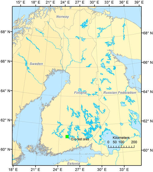
Fig. 1. Location of the test area.
The test area is a state-owned forest that is used as a training area for HAMK University of Applied Sciences. The field measurements employed in this study were carried out using fixed-radius (9.77 m) circular plots that were measured in 2010–2012. From each plot, all living tally trees with a breast-height diameter of at least 50 mm were measured. For each tally tree, the following variables were recorded: location, tree species, crown layer, diameter at breast height, height, and height of living crown. The geographic location of the field plots was measured with Trimble’s GEOXM 2005 Global Positioning System (GPS) device, and the locations were processed with local base station data, with an average error of approximately 0.6 m.
The following forest variables were calculated for sample plots on the basis of the tally trees: mean diameter, mean height, basal area, total volume of growing stock and volumes for tree species groups of pine, spruce and broadleaved trees. Mean height and diameter were calculated as the height and diameter of the basal area median tree. The volumes of individual tally trees were calculated using models by Laasasenaho (1982) which were based on tree species, stem diameter and height as independent variables.
The forests in the study area are dominated by coniferous tree species, mainly Scots pine (Pinus sylvestris L.) and Norway spruce (Picea abies [L.] Karst), and to a lesser degree, larches (Larix spp.). Of the deciduous species, birches (Betula pendula Roth and B. pubescens Ehrh.) are most common. Other, mainly non-dominant tree species present in the study area are aspen (Populus tremula) and grey alder (Alnus incana). Compared with forests typical to the region, the forests in the study area have relatively high variation in relation to the amount of growing stock, tree species composition and size of the trees. The characteristics of the principal forest variables in the field measurement data (covered by aerial imagery from 2011 and 2012) are presented in Table 1 and the growing stock volume distributions of the field data are presented in Fig. 2.
| Table 1. Average, maximum (Max) and standard deviation (Std) of field variables in the field data sets (for all variables: minimum = 0). | ||||||
| 2011 plots (81) | 2012 plots (165) | |||||
| Forest variable | Average | Max | Std | Average | Max | Std |
| Total volume, m3/ha | 215.8 | 529.4 | 110.9 | 213.6 | 653.6 | 119.2 |
| Volume of Scots pine, m3/ha | 76.0 | 314.3 | 80.4 | 77.9 | 314.3 | 80.8 |
| Volume of Norway spruce, m3/ha | 97.2 | 448.9 | 118.9 | 88.3 | 561.3 | 114.2 |
| Volume of broadleaved, m3/ha | 42.7 | 249.9 | 51.6 | 47.4 | 403.4 | 66.9 |
| Mean diameter, cm | 23.5 | 56.2 | 9.9 | 24.1 | 59.1 | 8.8 |
| Mean height, m | 20.2 | 34.7 | 7 | 20.6 | 34.7 | 6.3 |
| Basal area, m2/ha | 22.5 | 46.7 | 9.3 | 22.1 | 56.8 | 9.4 |
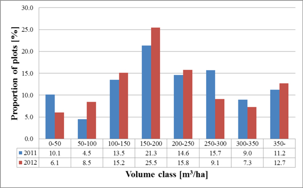
Fig. 2. The volume distribution of the dataset plots used with 2011 and 2012 image acquisition.
2.2 Aerial imagery
The aerial imagery used in this study was acquired in the summers of 2011 and 2012. We had airspace reservation for the study area up to altitude 600 m in order to be able to operate by autopilot and GPS, without the restriction of staying within visual line of sight. Different combinations of aircraft and camera equipment were utilised in the consecutive flight campaigns. In 2011, the aerial imagery was acquired using a combination of a Gatewing X100 UAV and a RICOH GR Digital III camera converted for acquiring colour-infrared imagery. The altitude used in the UAV flights was approximately 150 m above average ground elevation. The nominal distance between flight lines was 50 m. The area covered was approximately 350 ha, and there were 81 field sample plots in the photographed area. In 2012, the aerial imaging was carried out using a combination of C-Astral Bramor UAV and Olympus camera. The flight altitude used here was approximately 450 m above average ground elevation. The nominal distance between flight lines was 60 m. The area coverage was approximately 770 ha, and there were 165 field sample plots in the photographed area. The acquisition of aerial images in 2011 and 2012 was designed in a way that approximately 80 % sidelap and forward overlap was achieved in the inventory area. However, the actual within flight line stereo coverage varied depending on whether the UAV flew upwind or downwind, since both UAVs flew at constant airspeed. Thus, the interval between individual images was set to guarantee sufficient stereo-coverage when flying downwind.
The technical specifications of the camera sensors used in acquiring the aerial imagery are presented in Table 2. The locations of the true flight lines of the 2012 flight campaign as recorded by the UAV GPS receiver are illustrated in Fig. 3a, and the locations of field plots of 2011 and 2012 are shown in Fig. 3b.
| Table 2. Camera sensors fitted to UAVs. | ||
| Camera | Ricoh GR Digital III | Olympus E-420 |
| Sensor type | CCD | CMOS |
| Image sensor size | 17.3 mm ×13.0 mm | 17.3 mm × 13.0 mm |
| Image resolution | 3648 × 2736 pixels | 3648 × 2736 pixels |
| Field of View (FOV) | 65° × 51° | 38.1° × 29.1° |
| Pixel size | 4.74 µm | 4.74 µm |
| Groud sample distance* | 5.2 cm | 8.5 cm |
| Spectral bands** | 490 – 600 nm 600 – 700 nm 700 – 1000 nm | 490 – 600 nm 600 – 700 nm 700 – 1000 nm |
| Frame rate | 0.25 Hz | 0.5 Hz |
| Weight | 220 g | 380 g |
| Size | 109 × 60 × 26 mm | 129.5 × 91 × 53 mm |
| *At the applied flying altitude **Both Ricoh and Olympus had a blue cutting filter Schott GG495 which has a cut-off wavelength 495 nm. | ||
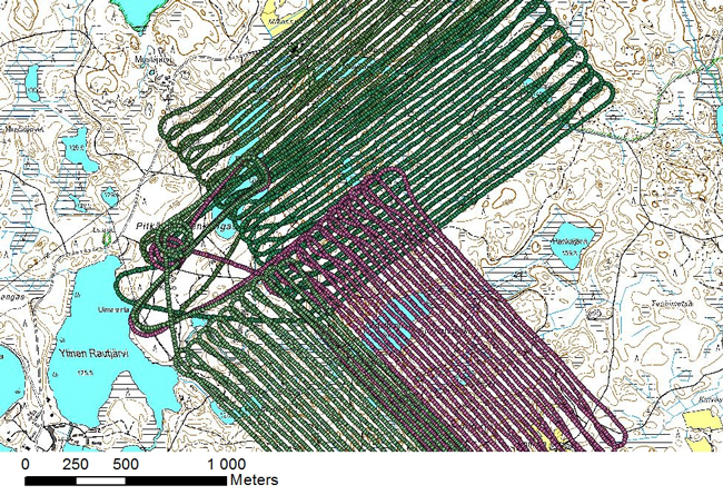
Fig. 3a. UAV flight lines of the 2012 photo acquisition. The take-off and landing site is located approximately 300 m north-east of Ylinen Rautjärvi (approach and descent curves made by the UAV prior to landing can be seen on the map).
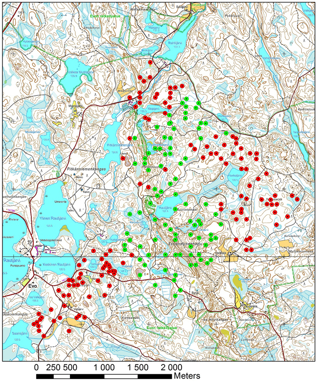
Fig. 3b. Location of field plots of 2011 (green) and 2012 (red).
Both UAV platforms used a catapult system for take-off. The Gatewing X100 was launched using an elastic bungee cord and the Bramor with a pneumatic system. Both UAVs require an open (treeless) strip of 100–200 metres in length (depending on the height of the surrounding trees) and a 30-metre width for gaining altitude after launch, before heading towards a pre-programmed flight route. The Gatewing X100 landed after flight by belly-landing at a pre-programmed point, requiring a treeless strip of approximately 200 × 40 metres for descent towards the landing point. The Bramor landed using a parachute system, after decreasing altitude by circling around a pre-programmed landing point it opened a parachute at a defined altitude, requiring only a small opening in the forest for landing. The modus operandi of both UAV platforms was found to be applicable for forest mapping operations in the tested conditions. However, the Bramor UAV combination of catapult take-off and parachute landing was considered technically preferable in Finnish forest conditions, mainly due to the parachute landing system, which was considered less prone to landing damage because at the touchdown moment the UAV vertical speed is low and horizontal velocity is close to zero. Furthermore, the parachute landing provides a higher number of potential spots for flight operations, since smaller open areas are needed in comparison to belly landing (where longer and wider approach areas without trees are required). The technical specifications of the UAV equipment are presented in Table 3.
| Table 3. UAV systems (Trimble unmanned aircraft systems 2013, Bramor UAS family 2013). | ||
| UAV | Gatewing X100 | C-Astral Bramor |
| Wing span (cm) | 100 | 230 |
| Fuselage length (cm) | 60 | 96 |
| Take-off weight (kg) | 2.2 | 4.2 |
| Payload | compact camera | 0.6 – 1.0 kg |
| Propulsion type | electric | electric |
| Take-off/landing | catapult launch/belly landing | catapult launch/parachute landing |
| Flight endurance (min) | 45 | 120 |
| Altitude ceiling (m) | 2500 | 5000 |
2.3 Image processing
2.3.1 Orthomosaic composite
The images were converted from the raw format of the cameras into 16-bit CIR images in TIF format using RapidToolbox software, and were radiometrically corrected for the effects of the sun and lens vignetting (light falloff) (PIEneering 2013b). After this preprocessing step, the EnsoMOSAIC photogrammetric software package was used to calculate the orthomosaics. A combined tie point search and photogrammetric bundle block adjustment (e.g. Krauss 1993) were carried out within automatic aerial triangulation, running the process repeatedly on six image pyramid levels, recalculating the results of increased accuracy on each pyramid level using the results of the previous level as starting point (MosaicMill 2013).
Ground control points were measured to account for systematic error of GPS and for synchronisation errors of GPS/camera trigger. Between 7 and 11 control points were used per flight, resulting in standard deviations of 2.2–19.5 m for X, 2.7–14.5 m for Y and 6.0–8.6 m for Z for each exposure station. These standard deviations show the size of the difference of the expected and calculated (true) exposure station XYZ, i.e. how accurately the autopilot has collected GPS coordinates and triggered the camera.
The results of the block adjustment were used to calculate sparse (internal) surface models for orthomosaicking. The sparse models were derived from the calculated elevations of the image tie and control points, thus the density of the tie and control points define the maximum density of the elevation models. For UAV data the tie points are usually calculated at 5–20 m distances, thus also the elevation model contains data at this density. The raster elevation models were resampled into 10 m cell size for all flights. It is important to point out that the sparse elevation models are used only to create orthomosaics, and not used to create dense point clouds or surface models addressed in the next chapter.
Orthomosaics were computed at a resolution of 10 cm, applying the surface models and the results of the triangulation. The optimal extraction of textural image features requires an appropriate scale between the image resolution and the size of the objects of interest (here tree crowns), and thus, excessively high or too coarse image resolutions are not useful for this purpose (e.g. Woodcock and Strahler 1987). For the extraction of digital raster image features, the image mosaic was resampled (nearest neighbour resampling used) to spatial resolutions of 20 and 50 cm.
2.3.2 Three demensional (3D) digital surface model (XYZ data)
Dense XYZ point clouds were computed using RapidTerrain software that utilises multi-image matching using variations of dense stereo-matching procedures with advanced probabilistic optimisation. The points were computed at image pyramid level 2, where the pixel size is double the original pixel size.
The point clouds were calculated at 10 cm intervals, with 5–10 Z observations for each XY point. A Z-value can be calculated for each stereo model covering a XY point, but in this case the number of stereo models was limited to 10 in order to have the best (the nearest) stereo models and in order to keep the processing times reasonable. RapidTerrain eliminates low correlation point matches (outliers) within the matching process, thus the remaining number of Z points was 10 or less for each XY. Out of these remaining points, the resulting Z-value is selected at the densest (most probable) Z, i.e. at Z where the most of the calculated Z-values lie (PIEneering 2013a).
In addition to the XYZ point data, the photogrammetric canopy height data were interpolated to a raster image format. The raster image pixel values of the height image were calculated using inverse-distance weighted interpolation based on the two nearest points. The output images were resampled to a spatial resolution similar to that of the orthoimages.
The DTM used in calculating canopy height values (above ground) was based on laser scanning in 2006. ALS data was acquired from a flying altitude of 1900 m with a density of 1.8 returned pulses per square metre. A raster DTM with 1 meter resolution was derived by inverse distance weighting of the elevation values of ALS ground returns.
2.4 Extraction of the aerial photograph features
The remote sensing features were extracted for each sample plot from a square window centred on the sample plot. The size of the window was set as 19.4 × 19.4 m (when using raster data with a spatial resolution of 20 cm) or 19.5 × 19.5 m (when using raster data with a spatial resolution of 50 cm). The size was set to correspond to the size of the field measurement plot (radius 9.77), and besides, the extraction window is constrained by the GRASS software applied for calculating textural features requiring an uneven number of pixel rows and columns. The following features were extracted from the aerial photographs and rasterised point height data:
1. Spectral averages (AVG) of orthoimage pixel values of NIR, R & G channels
2. Standard deviations (STD) of orthoimage pixel values of NIR, R & G channels
3. Textural features based on co-occurrence matrices of orthoimage pixel values of NIR, R, G & H channels (Haralick 1979; Haralick et al. 1973; GRASS GIS 7.0. 2013 )
a. Sum Average (SA)
b. Entropy (ENT)
c. Difference Entropy (DE)
d. Sum Entropy (SE)
e. Variance (VAR):
f. Difference Variance (DV)
g. Sum Variance (SV)
h. Angular Second Moment (ASM, also called Uniformity)
i. Inverse Difference Moment (IDM, also called Homogeneity)
j. Contrast (CON)
k. Correlation (COR)
l. Information Measures of Correlation (MOC)
E.g. COR_R = correlation of red channel
The following features were extracted from photogrammetric (XYZ format) 3D point data (Næsset 2004; Packalén and Maltamo 2006, 2008):
1. Average value of H of vegetation points [m] (HAVG)
2. Standard deviation of H of vegetation points [m] (HSTD)
3. H where percentages of vegetation points (0%, 5%, 10%, 15%, ... , 90%, 95%, 100%) were accumulated [m] (e.g. H0, H05,...,H95, H100)
4. Coefficient of variation of H of vegetation points [%] (HCV)
5. Proportion of vegetation points [%] (VEG)
6. Canopy densities corresponding to the proportions points above fraction no. 0, 1,..., 9 to total number of points (D0, D1,…, D9)
7. Proportion of vegetation points having H greater or equal to corresponding percentile of H (i.e. P20 is the proportion of points having H>= H20) (%) *
8. Ratio of the number of vegetation points to the number of ground points
where:
H = height above ground
vegetation point = point with H > = 2 m
ground point = other than vegetation point
*the range of H was divided into 10 fractions (0, 1, 2,…, 9) of equal distance
In principle, the extraction of the 3D point features is similar to the extraction method applied for ALS features, but while ALS is true 3D in the sense that it allows multiple Z returns from a single XY point, photogrammetric data have only one Z-value for each point, not allowing any features below overhanging objects.
2.5 Feature selection and k-nn estimation
The k-nearest neighbour (k-nn) method was used for the estimation of the forest variables. The estimated stand variables were total volume of growing stock, the volumes of Scots pine, Norway spruce and deciduous species, basal area, mean diameter and mean height. Different values of k were tested in the estimation procedure. In the k-nn estimation (e.g. Kilkki and Päivinen 1987; Muinonen and Tokola 1990; Tomppo 1991), the Euclidean distances between the sample plots were calculated in the n-dimensional feature space, where n stands for the number of remote sensing features used. The stand variable estimates for the sample plots were calculated as weighted averages of the stand variables of the k-nearest neighbours (Eq. 1). Weighting by inverse squared Euclidean distance in the feature space was applied (Eq. 2) for diminishing the bias of the estimates (Altman 1992). Without weighting, the k-nn method often causes undesirable averaging in the estimates, especially in the high end of the stand volume distribution, where the reference data is typically sparse.

where
![]() = estimate for variable y
= estimate for variable y
![]() = measured value of variable y in the ith nearest neighbour plot
= measured value of variable y in the ith nearest neighbour plot

di = Euclidean distance (in the feature space) to the ith nearest neighbour plot
k = number of nearest neighbours
g = parameter for adjusting the progression of weight with increasing distance*
*(1–2 depending on the variable)
The accuracy of the estimates was calculated via leave-one-out cross-validation by comparing the estimated forest variable values with the measured values (ground truth) of the field plots. The accuracy of the estimates was measured in terms of the relative root mean square error (RMSE) (Eq. 3).

where:
![]() = measured value of variable y on plot i
= measured value of variable y on plot i
![]() = estimated value of variable y on plot i
= estimated value of variable y on plot i
![]() = mean of the observed values
= mean of the observed values
n = number of plots.
The remote sensing datasets encompassed a total of 42 aerial photograph features, 12 features from rasterised canopy height data and 35 3D point features. All aerial image and point features were scaled to a standard deviation of 1. This was done because the original features had very diverse scales of variation. Without scaling, variables with wide variation would have had greater weight in the estimation, regardless of their capability for estimating the forest attributes.
The extracted feature set was large, presenting a high-dimensional feature space for the k-nn estimation. In order to avoid the problems of the high-dimensional feature space, i.e. the ‘curse of dimensionality’, which is inclined to complicate the nearest neighbour search (e.g. Beyer et al. 1999; Hinneburg et al 2000), the dimensionality of the data was reduced by selecting a subset of features with the aim of good discrimination ability. The selection of the features was performed with a genetic algorithm (GA) -based approach, implemented in the R language by means of the Genalg package (R Core Team 2012; Willighagen 2005). The evaluation function of the genetic algorithm was employed to minimise the RMSEs of k-nn estimates for each variable in leave-one-out cross-validation. The feature selection was carried out separately for each forest attribute.
In the selection procedure, the population consisted of either 300 or 400 binary chromosomes, and the number of generations was 100 or 200. We carried out 13 feature-selection runs for each attribute to find the feature set that returned the best evaluation value. In selecting the feature weights, floating point chromosomes with values in the range of 0–1 were used, and the number of generations was set to 400. Otherwise the selection procedure was similar to the feature selection. The values for parameters k and g (Eq. 1 and 2) were selected during the test runs. Number of nearest neighbors varied between 2, 3 and 4 depending on the variable, and g was between 1–2.
3 Results
For all the estimated variables, the 3D-features were in the majority among the selected features in relation to the aerial image features. Among the aerial image features, textural features (i.e. Haralick features or standard deviations of image pixel values) were selected most often. Spectral aerial image features were very seldom represented among the selected features. The results of feature selections for two main estimated forest variables, stand height and total volume of growing stock, are presented in Table 4 (results are shown for both tested image data resolutions; 20 and 50 cm).
| Table 4. The feature combinations selected by GA for estimating forest variables based on data of 20 and 50 cm spatial resolutions (DBH = diameter at breast height, v. = volume of growing stock, for feature abbreviations see section 2.4). | |
| Height (20 cm) | STD_G, H05, H30, H80, H85, H95, HCV, VEG, P60, IDM_R, MOC_G, MOC_H, SV_H |
| Height (50 cm) | STD_G, HAVG, H30, H40, H85, H95, H100, P40, DV_R, MOC_G, MOC_H, SV_H |
| DBH (20 cm) | HSTD, H0, H90, H95, H100, P20, P60, MOC_NIR, ASM_R, ENT_G, DE_H, MOC_H |
| DBH (50 cm) | H30, H90, H100, P60, P95, SA_G, COR_H, MOC_H, SA_H |
| Basal area (20 cm) | HAVG, H20, H40, H80, H90, D3, ENT_NIR, SV_R, ASM_G, ASM_H, CON_H |
| Basal area (50 cm) | HSTD, H20, H40, H70, H80, D2, P40, DE_NIR, SV_R, CON_H, DE_H, MOC_H |
| V. total (20 cm) | HSTD, H10, H70, H80, H85, H90, H95, D0, P60, SA_R, CON_H, DV_H |
| V. total (50 cm) | HAVG, HSTD, H20, H30, H90, P20, DE_NIR, SA_R, ASM_H, CON_H |
| V. pine (20 cm) | MEAN_NIR, H20, H80, H85, H95, D2, D6, D9, P60, COR_NIR, DE_NIR, IDM_H, SV_H |
| V. pine (50 cm) | STD_G, H20, H40, H80, H85, H95, HCV, VEG, P80, PCG, DV_NIR, SE_R, CON_G, DV_G, SE_G, IDM_H, MOC_H |
| V. spruce (20 cm) | MEAN_NIR, HSTD, H40, H70, H100, D3, P80, IDM_H |
| V. spruce (50 cm) | MEAN_NIR, STD_G, HSTD, H20, H050, H80, H95, HCV, D3, ASM_R, IDM_R, ASM_G, DE_G, CON_H, IDM_H, MOC_H |
| V. broadleaf (20 cm) | HSTD, H0, H40, H80, H90, D2, D8, PGH, SV_NIR, COR_G, ASM_H, IDM_H, SA_H, VAR_H |
| V. broadleaf (50 cm) | STD_R, H050, H85, H100, D8, P95, ASM_NIR, ASM_R, COR_R, SA_R, MOC_G, CON_H, COR_H, MOC_H, VAR_H |
The imagery from 2011 resulted in better estimation accuracy than the imagery from 2012, mainly due to the better quality of the image material (camera parameters of 2012 imagery were not best suited for light conditions). When inspected visually, the 2011 imagery had better radiometric quality than the imagery of 2012. Comparing the datasets from consecutive years showed, however, that there was considerably lower relative RMSE for volumes of pine and spruce in the 2012 data set when taking into account the lowest relative RMSE values calculated from the 2012 data set divided by flight areas. This indicates that there is high variation in the quality of image material between different flights, which suggests that changes have occurred in the photographing conditions between the flights, mainly due to changes in weather and/or solar illumination, which have not been properly taken into account in the acquisition of the images. These variations have probably been the main factor in the reduced data quality in 2012. The best results are mainly from Flight 3. When comparing results from the entire 2011 data and data from Flight 3 in 2012, relative RMSEs of height are lower in the latter data set, whereas the 2011 data set performed better in estimating total volume. When all flights are considered, the 2011 data gave better results in all tested forest variables.
When testing the effect of the spatial resolution of orthoimages, the results indicate little difference in the estimation accuracy with the tested resolutions of 20 and 50 cm on both orthoimages and DSM. When comparing the 20 and 50 cm resolution data sets from the 2011 photo acquisition, the mean stand height estimates as well as those of the volumes of spruce and broadleaved trees were more accurate in the 0.2 m resolution data set, while in other variables the coarser resolution set gave a better estimate for total volume and in all the runs for basal area. However, for all tested forest variables, the effect of spatial resolution was relatively small. The estimation accuracy for the tested forest variables with 2011 imagery (using resolutions of 20 and 50 cm) is presented in Fig. 4. The comparison between results of 2011 and 2012 data sets (with similar resolutions) is presented in Fig. 5.
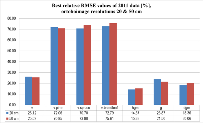
Fig. 4. Relative RMSE values [%] for estimated forest variables at sample plot level (2011 data, orthoimage resolutions 20 and 50 cm). Variables: v = volume, g = basal area, hgm/dgm = mean height/diameter (as measured from basal-area weighted median tree).
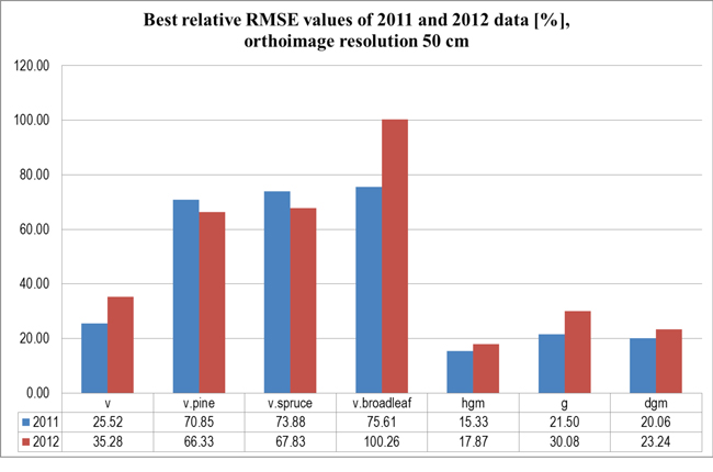
Fig. 5. Relative RMSE values [%] for estimated forest variables at sample plot level (2011 and 2012 data, orthoimage resolution 50 cm).
4 Discussion
The performance of the UAS system in practical aerial image acquisition was good, despite some difficult flying conditions in the area of operation. For example, during the flights the UAV was occasionally affected by forceful gusts of crosswind at speeds of 10–15 m/s. Still the UAV autopilot was capable of holding the UAV position in the programmed flight route so that there were no gaps in the image coverage. On the other hand, due to various teething problems in operating the UAV and camera equipment, there were some shortcomings concerning the image quality and the amount of image coverage. For example, in the 2012 imaging campaign the settings of camera parameters were found not optimal for the prevalent light conditions, and furthermore, the Bramor UAV was acquired very recently, and little experience had been gathered of operating the system at that time. Thus, it is possible that the full potential of the method was not achieved.
When assessing the features selected for the estimation task by GA, the list of selected features was markedly similar to those typically applied when using ALS data and conventional aerial imagery (e.g. Tuominen and Haapanen 2011). This supports the assumption that the information content of photogrammetric CHM is similar to that of ALS-based canopy height data. Cross-validating the estimation results indicated that the estimation accuracy at sample plot level for the tested forest variables (total volume of growing stock, volumes of pine, spruce and broadleaved trees, basal area, mean height and diameter) was very similar to or slightly better than the results of earlier estimation tests with a combination of ALS and aerial images in the same study area and using similar field material (e.g. Tuominen and Haapanen 2011; Holopainen et al. 2008). In addition to the different way of producing 3D point data, the main difference to the aforementioned earlier studies is that in this study the number of available field reference plots was considerably lower. Due to the fact that the field reference data set here was markedly smaller than in the aforementioned studies, the results are not entirely comparable. Typically, in inventories where non-parametric estimators such as k-nn have been applied, relatively large set of reference plots have been used (up to 600–800), depending on the purpose of the inventory and the variation within the inventory area. Yet a number of studies focusing on ALS-based forest inventories have noted that appropriate inventory results can be achieved using a relatively low number of reference plots, when those plots are selected in a suitable way (e.g. Gobakken and Næsset 2008; Junttila et al. 2008; Maltamo et al. 2011). Based on these studies, even 60–100 field reference plots would be enough for reaching relatively high estimation accuracy for variables such as the total volume of growing stock, whereas the addition of further plots does not significantly improve the estimation accuracy. On the other hand, in the case of operational forest inventories, it is typical that a high number of inventory variables to be estimated (such as volumes of various tree species) may require a significantly higher number of reference plots, since the estimation problem is more complicated (as in the case of proportions of various tree species). The selection of remote sensing features is usually a compromise between the estimation accuracies of several inventory variables. In such a case, it is very likely that a significantly higher number of field reference plots will be required for sufficiently covering the relevant variation over the variables of interest. From this perspective, the performance of combination photogrammetric 3D and image data applied in this study has been very good.
Järnstedt et al. (2012) have tested, in the same study area, a photogrammetric canopy surface model based on more conventional aerial stereo imagery, which was acquired using an aircraft-mounted Microsoft UltracamXp imaging sensor from a considerably higher imaging altitude. Compared to the results by Järnstedt et al. (2012), the estimation accuracy of forest variables was considerably better in this study. Also, when visually inspecting the 3D canopy data of this study and that of Järnstedt et al., the canopy model of this study appears to be of considerably higher quality and more detailed. There are some probable reasons for the differences: the considerably lower imaging altitude used in this study allowing higher spatial resolution, the greater stereo overlap and furthermore, different software used for building the digital surface models, where recent development in digital photogrammetry may have brought more sophisticated algorithms and, thereby, more detailed or more realistic surface models.
In other studies using the area-based estimation method with test material from similar conditions, estimates of stand height with relative RMSE as low as 8–9% have been achieved with the help of ALS data, which indicates distinctly higher performance of the ALS data compared to the photogrammetric data used here (e.g. Vastaranta et al. 2012). Since the ALS data may have several Z values for each point and photogrammetric data have only one Z-value, the informational content of ALS is higher, and also the content of extracted point features is slightly different. Part of the difference in the estimation accuracy may be due to the different variations of forest variables in the test data sets and the coverage of the reference plots in relation to the full distribution of forest variables in the test data. For example, there may be a relatively low number of available reference plots in the high end of the distribution, which causes bias in the estimates due to the fact that k > 1 is typically used in k-nn estimation. On the other hand, the shape of the tree crowns in photogrammetric DSM differs from that of laser-based DSM, depending on the properties of the software used for producing the DSM. Photogrammetric DSMs often fail to accurately represent the complex morphology of the canopy surface, whereas at least the near nadir geometry of ALS acquisition enables the detailed canopy features to be reconstructed in the canopy surface model. It has also been noted that ALS is generally more successful than photogrammetry in detecting canopy gaps (e.g. Andersen et al. 2003). On the other hand, ALS also has limited capability for detecting and measuring the accurate elevation of a conifer tree top (Jung et al. 2011).
5 Conclusions
The tested combination of orthoimagery and DSM derived from UAV-borne camera images was found to be well suited to the estimation of forest stand variables.
The accuracy of forest estimates based on the data combination was similar to that of the combination of ALS and digital aerial imagery using similar estimation methodology.
The tested method has potential in stand level forest inventory. In acquiring large area image coverage, conventional aerial imaging is likely to remain more efficient than image acquisition based on small UAVs.
In addition to technical problems, there are points in aviation legislation that should be revised in order to enhance the operational feasibility of the presented methodology.
Acknowledgements
This study has received a major part of its funding from the Finnish Funding Agency for Technology and Innovation (TEKES). In addition, the authors wish to thank the following partners for their support in this project: the Finnish defence forces, Tornator Oy, Metsähallitus, Suonentieto Oy and Millog Oy. Furthermore, this study would not have been possible without the technical support of East Lapland Vocational College and PIEneering Oy, who provided the UAS equipment and other technical hardware as well as their valuable know-how for the use of this project, and we wish to express our special gratitude to J. Nykänen and M. Sippo. Finally, we would like to thank those students at HAMK University of Applied Sciences who participated in the fieldwork of this study for their valuable contribution.
References
Altman N.S. (1992). An introduction to kernel and nearest-neighbor nonparametric regression. The American Statistician 46(3): 175–185.
Andersen H.-E., McGaughey R.J., Carson W., Reutebuch S., Mercer B., Allan J. (2003). A comparison of forest canopy models derived from LIDAR and INSAR data in a Pacific Northwest conifer forest. International Archives of Photogrammetry and Remote Sensing, vol. XXXIV-3/W13. 7 p. http://www.isprs.org/proceedings/XXXIV/3-W13/papers/Andersen_ALSDD2003.pdf.
Anderson K., Gaston K.J. (2013). Lightweight unmanned aerial vehicles will revolutionize spatial ecology. Frontiers in Ecology and the Environment 11(3): 138–146. http://dx.doi.org/10.1890/120150.
Axelsson P. (1999). Processing of laser scanner data – algorithms and applications. ISPRS Journal of Photogrammetry and Remote Sensing 54(2–3): 138–147. http://dx.doi.org/10.1016/S0924-2716(99)00008-8.
Axelsson P., 2000. DEM generation from laser scanner data using adaptive TIN models. International Archives of Photogrammetry and Remote Sensing 33(B4): 110–117.
Baltsavias E.P. (1999). A comparison between photogrammetry and laser scanning. ISPRS Journal of Photogrammetry and Remote Sensing 54(2–3): 83–94. http://dx.doi.org/10.1016/S0924-2716(99)00014-3.
Baltsavias E., Gruen A., Zhang L., Waser L.T. (2008). High quality image matching and automated generation of 3D tree models. International Journal of Remote Sensing 29(5): 1243–1259. http://dx.doi.org/10.1080/01431160701736513.
Beyer K.S., Goldstein J., Ramakrishnan R., Shaft U. (1999). When is ‘nearest neighbor’ meaningful? In: Beeri C., Buneman P. (eds.). Proceedings of the 7th international conference on database theory (ICDT), Jerusalem, 10–12 January. p. 217–235. http://dx.doi.org/10.1007/3-540-49257-7_15.
Bohlin J., Wallerman J., Fransson J.E.S. (2012). Forest variable estimation using photogrammetric matching of digital aerial images in combination with a high-resolution DEM. Scandinavian Journal of Forest Research 27(7): 692–699. http://dx.doi.org/10.1080/02827581.2012.686625.
Bramor UAS family (2013). http://www.c-astral.com/en/products/bramor-c4eye.
Gobakken T., Næsset E. (2008). Assessing effects of laser point density, ground sampling intensity, and field plot sample size on biophysical stand properties derived from airborne laser scanner data. Canadian Journal of Forest Research 38: 1095–1109. http://dx.doi.org/10.1139/X07-219.
GRASS Development Team (2013). GRASS GIS 7.0.svn reference manual. http://grass.osgeo.org/grass70/manuals/index.html. [Cited 15 November 2013].
Gruen A., Zhang L. (2003). Automatic DTM generation from TLS data. In: Gruen A., Kahman H. (eds.). Optical 3-D measurement techniques VI, Vol. I. p. 93–105. ISBN 3-906467-43-0.
Haala N., Hastedt H., Wolf K., Ressl C., Baltrusch S. (2010). Digital photogrammetric camera evaluation – generation of digital elevation models. The Journal of Photogrammetry, Remote Sensing and Geoinformation Processing 2010(2): 98–115. http://dx.doi.org/10.1127/1432-8364/2010/0043.
Haralick R.M. (1979). Statistical and structural approaches to texture. Proceedings of the IEEE 67(5): 786–804. http://dx.doi.org/10.1109/PROC.1979.11328.
Haralick R.M., Shanmugam K., Dinstein I. (1973). Textural features for image classification. IEEE Transactions on Systems, Man and Cybernetics SMC-3(6): 610–621. http://dx.doi.org/10.1109/TSMC.1973.4309314.
Hinneburg A., Aggarwal C.C., Keim D.A. (2000). What is the nearest neighbor in high dimensional spaces? In: El Abbadi A., Brodie M.L., Chakravarthy S., Dayal U., Kamel N., Schlageter G., Whang K.-Y. (eds.). Proceedings of the 26th very large data bases (VLDB) conference, September 10–14, Cairo, Egypt. p. 506–515.
Holopainen M., Haapanen R., Tuominen S., Viitala R. (2008). Performance of airborne laser scanning- and aerial photograph-based statistical and textural features in forest variable estimation. In: Hill R.A., Rosette J., Suárez J. (eds.). Proceedings of SilviLaser 2008: 8th international conference on lidar applications in forest assessment and inventory, 17–19 September, Heriot-Watt University, Edinburgh. p. 105–112.
Hyyppä J., Pyysalo U., Hyyppä H., Samberg A. (2000). Elevation accuracy of laser scanning-derived digital terrain and target models in forest environment. Proceedings of EARSeL-SIG-Workshop LIDAR, 16–17 June, Dresden. p. 139–147.
Järnstedt J., Pekkarinen A., Tuominen S., Ginzler C., Holopainen M., Viitala R. (2012). Forest variable estimation using a high-resolution digital surface model. ISPRS Journal of Photogrammetry and Remote Sensing 74: 78–84. http://dx.doi.org/10.1016/j.isprsjprs.2012.08.006.
Jung S.-E., Kwak D.-A., Park T., Lee W.-K., Yoo S. (2011). Estimating crown variables of individual trees using airborne and terrestrial laser scanners. Remote Sensing 3: 2346–2363. http://dx.doi.org/10.3390/rs3112346.
Junttila V., Maltamo M., Kauranne T. (2008). Sparse Bayesian estimation of forest stand characteristics from ALS. Forest Science 54: 543–552.
Kilkki P., Päivinen R. (1987). Reference sample plots to combine field measurements and satellite data in forest inventory. Department of Forest Mensuration and Management, University of Helsinki, Research Notes 19. p. 210–215.
Koh L.P., Wich S.A. (2012). Dawn of drone ecology: low-cost autonomous aerial vehicles for conservation. Tropical Conservation Science 5(2): 121–132.
Krauss K. (1993). Photogrammetry, Volume I. Ferd. Dummlers Verlag, Bonn, Germany. 397 p. ISBN 3-427-786846.
Kumpula M. (2013). UAV-lennokin hyödynnettävyys ilmakuvakartan teossa. Rovaniemi University of Applied Sciences, Rovaniemi, Finland. 43 p. http://www.theseus.fi/bitstream/handle/10024/59910/Kumpula_Mikko.pdf. [Cited 18 December 2013].
Laasasenaho J. (1982). Taper curve and volume functions for pine, spruce and birch. Communicationes Instituti Forestalis Fenniae 108: 1–74.
Lisein J., Pierrot-Deseilligny M., Bonnet S., Lejeune P. (2013). A photogrammetric workflow for the creation of a forest canopy height model from small unmanned aerial system imagery. Forests 4: 922–944. http://dx.doi.org/10.3390/f4040922.
Maltamo M., Malinen J., Packalén P., Suvanto A., Kangas J. (2006). Nonparametric estimation of stem volume using airborne laser scanning, aerial photography, and stand-register data. Canadian Journal of Forest Research 36(2): 426–436. http://dx.doi.org/10.1139/x05-246.
Maltamo M., Bollandsås O.M., Næsset E., Gobakken T., Packalén P. (2011). Different plot selection strategies for field training data in ALS-assisted forest inventory. Forestry 84(1): 23–31. http://dx.doi.org/10.1093/forestry/cpq039.
MosaicMill (2013). EnsoMOSAIC image processing – user’s guide. Version 7.5. MosaicMill Ltd, Vantaa, Finland. 105 p.
Muinonen E., Tokola T. (1990). An application of remote sensing for communal forest inventory. In: Proceedings from SNS/IUFRO workshop in Umeå, 26–28 Feb. Remote Sensing Laboratory, Swedish University of Agricultural Sciences, Report 4. p. 35–42.
Næsset E. (2002). Predicting forest stand characteristics with airborne scanning laser using a practical two-stage procedure and field data. Remote Sensing of Environment 80(1): 88–99. http://dx.doi.org/10.1016/S0034-4257(01)00290-5.
Næsset E. (2004). Practical large-scale forest stand inventory using a small airborne scanning laser. Scandinavian Journal of Forest Research 19(2): 164–179. http://dx.doi.org/10.1080/02827580310019257.
Ojala J. (2011). Miehittämättömien ilma-alusten käyttö ilmakuvauksessa. Rovaniemi University of Applied Sciences, Rovaniemi, Finland. 33 p. http://www.theseus.fi/bitstream/handle/10024/26549/Ojala_Jaska.pdf. [Cited 20 December 2013].
Packalén P., Maltamo M. (2006). Predicting the plot volume by tree species using airborne laser scanning and aerial photographs. Forest Science 52(6): 611–622.
Packalén P., Maltamo M. (2007). The k-MSN method in the prediction of species-specific stand attributes using airborne laser scanning and aerial photographs. Remote Sensing of Environment 109: 328–341. http://dx.doi.org/10.1016/j.rse.2007.01.005.
Packalén P., Maltamo M. (2008). Estimation of species-specific diameter distributions using airborne laser scanning and aerial photographs. Canadian Journal of Forest Research 38: 1750–1760. http://dx.doi.org/10.1139/X08-037.
PIEneering (2013a). RapidTerrain user’s guide, version 1.2.0. PIEneering Ltd, Helsinki, Finland. 57 p.
PIEneering (2013b). RapidToolbox user’s guide, version 2.2.4. PIEneering Ltd, Helsinki, Finland. 29 p.
Pyysalo U. (2000). A method to create a three-dimensional forest model from laser scanner data. The Photogrammetric Journal of Finland 17(1): 34–42.
R Core Team (2012). R: a language and environment for statistical computing. R Foundation for Statistical Computing, Vienna, Austria. ISBN 3-900051-07-0. http://www.R-project.org/. [Cited 4 June 2012].
Salamí E., Barrado C., Pastor E. (2014). UAv flight experiments applied to the remote sensing of vegetated areas. Remote Sensing 6: 11051–11081. http://dx.doi.org/10.3390/rs61111051.
St-Onge B, Vega C., Fournier R.A., Hu Y. (2008). Mapping canopy height using a combination of digital stereo-photogrammetry and lidar. International Journal of Remote Sensing 29: 3343–3364. http://dx.doi.org/10.1080/01431160701469040.
Tomppo E. (1991). Satellite image-based national forest inventory of Finland. International Archives of Photogrammetry and Remote Sensing 1991(28): 419–424.
Törmä M. (2000). Estimation of tree species proportions of forest stands using laser scanning. International Archives of Photogrammetry and Remote Sensing XXXIII(Part B7): 1524–1531.
Trimble unmanned aircraft systems for surveying and mapping (2013). http://uas.trimble.com/. [Cited 18 Nov 2013].
Tuominen S., Haapanen R. (2011). Comparison of grid-based and segment-based estimation of forest attributes using airborne laser scanning and digital aerial imagery. Remote Sensing 3(5): 945–961 (Special Issue ‘100 Years ISPRS – Advancing Remote Sensing Science’). http://dx.doi.org/10.3390/rs3050945.
Vastaranta M., Kankare V., Holopainen M., Yu X., Hyyppä J., Hyyppä H. (2012). Combination of individual tree detection and area-based approach in imputation of forest variables using airborne laser data. ISPRS Journal of Photogrammetry and Remote Sensing 67: 73–79. http://dx.doi.org/10.1016/j.isprsjprs.2011.10.006.
Waser L.T., Ginzler C., Kuechler M., Baltsavias E., Hurni L. (2011). Semi-automatic classification of tree species in different forest ecosystems by spectral and geometric variables derived from Airborne Digital Sensor (ADS40) and RC30 data. Remote Sensing of Environment 115(1): 76–85. http://dx.doi.org/10.1016/j.rse.2010.08.006.
Watts A.C., Ambrosia V.G., Hinkley E.A. (2012). Unmanned aircraft systems in remote sensing and scientific research: classification and considerations of use. Remote Sensing 4(6): 1671–1692. http://dx.doi.org/10.3390/rs4061671.
White J.C., Wulder M.A., Vastaranta M., Coops N.C., Pitt D., Woods M. (2013). The utility of image-based point clouds for forest inventory: a comparison with airborne laser scanning. Forests 4: 518–536. http://dx.doi.org/10.3390/f4030518.
Willighagen E. (2005). Genalg: R based genetic algorithm, R package version 0.1.1. http://CRAN.R-project.org/package=genalg. [Cited 4 Feb 2012].
Woodcock C.E., Strahler A.H. (1987). The factor of scale in remote sensing. Remote Sensing of Environment 21(3): 311–332. http://dx.doi.org/10.1016/0034-4257(87)90015-0.
Total of 54 references.
