Tropical forest canopy cover estimation using satellite imagery and airborne lidar reference data
Korhonen L., Ali-Sisto D., Tokola T. (2015). Tropical forest canopy cover estimation using satellite imagery and airborne lidar reference data. Silva Fennica vol. 49 no. 5 article id 1405. https://doi.org/10.14214/sf.1405
Highlights
- The fusion of airborne lidar data and satellite images enables accurate canopy cover mapping
- The zero-and-one inflated beta regression is demonstrated in large area estimation
- Forest/non-forest classification should be done directly, for example by using logistic regression.
Abstract
The fusion of optical satellite imagery, strips of lidar data and field plots is a promising approach for the inventory of tropical forests. Airborne lidars also enable an accurate direct estimation of the forest canopy cover (CC), and thus a sample of lidar strips can be used as reference data for creating CC maps which are based on satellite images. In this study, our objective was to validate CC maps obtained from an ALOS AVNIR-2 satellite image wall-to-wall, against a lidar-based CC map of a tropical forest area located in Laos. The reference CC values which were needed for model training were obtained from a sample of four lidar strips. Zero-and-one inflated beta regression (ZOINBR) models were applied to link the spectral vegetation indices derived from the ALOS image with the lidar-based CC estimates. In addition, we compared ZOINBR and logistic regression models in the forest area estimation by using >20% CC as a forest definition. Using a total of 409 217 30 × 30 m population units as validation, our model showed a strong correlation between lidar-based CC and spectral satellite features (root mean square error = 12.8%, R2 = 0.82). In the forest area estimation, a direct classification using logistic regression provided better accuracy than the estimation of CC values as an intermediate step (kappa = 0.61 vs. 0.53). It is important to obtain sufficient training data from both ends of the CC range. The forest area estimation should be done before the CC estimation, rather than vice versa.
Keywords
logistic regression;
beta regression;
forest area;
international forest definition;
ALOS AVNIR-2;
vegetation index
-
Korhonen,
University of Eastern Finland, School of Forest Sciences, P.O. Box 111, FI-80101 Joensuu, Finland; (current) University of Helsinki, Department of Forest Sciences, P.O. Box 27, FI-00014 University of Helsinki, Finland
 http://orcid.org/0000-0002-9352-0114
E-mail
lauri.z.korhonen@helsinki.fi

- Ali-Sisto, University of Eastern Finland, School of Forest Sciences, P.O. Box 111, FI-80101 Joensuu, Finland E-mail dheikkil@student.uef.fi
- Tokola, University of Eastern Finland, School of Forest Sciences, P.O. Box 111, FI-80101 Joensuu, Finland. E-mail timo.tokola@uef.fi
Received 9 June 2015 Accepted 18 August 2015 Published 1 September 2015
Views 134479
Available at https://doi.org/10.14214/sf.1405 | Download PDF

Abbreviations
| ALOS | Advanced Land Observing Satellite |
| ARVI | Atmospherically Resistant Vegetation Index |
| AVNIR-2 | Advanced Visible and Near Infrared Radiometer - type 2 |
| CC | Canopy Cover |
| FCI | First echo Cover Index |
| LSO-CV | Leave-Strip-Out Cross Validation |
| NDVI | Normalized Difference Vegetation Index |
| RMSE | Root Mean Square Error |
| SR | Simple Ratio |
| ZOINBR | Zero-and-One Inflated Beta Regression |
1 Introduction
There are considerable uncertainties in undertaking estimates of a tropical forest area and its changes (Achard et al. 2014). Observing changes in the forest canopy cover (CC) is critical in the monitoring of forest areas because CC is the main criterion in the international definition of forest. Forest is defined internationally as “land spanning more than 0.5 hectares with trees higher than 5 meters and a canopy cover of more than 10 percent” (FAO 2005). Areas under reforestation which have yet to reach a canopy cover of 10 percent are included, however national minimum CC limits for forest can range from 10 to 30 percent (UNFCCC 2001). Thus, deforestation can be defined as the reduction of CC below the minimum canopy cover criterion, and any smaller decrease may indicate forest degradation.
Canopy cover is defined as the proportion of the forest floor which is covered by the vertical projection of the tree crowns, so that only the gaps between individual crowns are observed (Jennings et al. 1999; Gschwantner et al. 2009). Thus the CC of a closed-canopy tropical forest is typically close to 100%. An unbiased estimation of CC requires that the area of interest is covered by vertical point observations, where the proportion of between-crown gaps is recorded (Korhonen et al. 2006). However, field measurements of CC are laborious and expensive, and in addition, many tropical and boreal forest areas are difficult to access.
Airborne small-footprint lidar (light detection and ranging) sensors can provide CC estimates that are comparable to the most accurate field-based estimates (Korhonen et al. 2011; Gatziolis 2012). The fraction of pulses that penetrate to the ground without interacting with the foliage provides an estimate of CC that is similar to field-based dot count estimates, because the view geometry of airborne lidars is close to vertical. For example, Korhonen et al. (2011) found that the absolute root mean square error (RMSE) of lidar-based estimates was less than 5% when only the echoes from the closest scan strip were used.
A restriction of airborne lidar use is that continuous, nationwide inventories are too expensive to conduct and maintain. Optical satellite imagery is better suited for this task, as it is more affordable and new images are frequently available. Most forest inventories in developing countries utilize medium resolution (20–30 m) satellite images that are combined with field plots and higher resolution (< 2 m) remote sensing data. The integration of satellite images, airborne laser scanning and field measurements has recently been proposed as a method for creating regional carbon stock estimates (Asner et al. 2010). Multi-phase inventory designs that utilize strips of lidar data to estimate the biomass of large areas have also been developed (McRoberts et al. 2014). Such inventories are inexpensive because wall-to-wall lidar coverage is not needed. Lidar strips can also be used to provide auxiliary information in the interpretation of lower resolution images (Andersen et al. 2011; Strunk et al. 2014), and if inventories relying on samples derived from lidar became widely used, they would also provide training data for CC mapping using satellite images.
The results obtained in the estimation of CC from optical satellite images have been reasonably good (R2 ≈ 0.60, RMSE 6–26%) (Gemmell et al. 2001; Franklin et al. 2003; Wolter et al. 2009), except for those concerning tropical forests (R2 = 0.29) (Koy et al. 2005). However, in many studies the field measurements of CC have been obtained using imprecise or biased methods, and this makes any accuracy assessment of remotely sensed CC estimates difficult. The main advantage of CC estimates derived from airborne lidar is that the data are accurate and consistent within each scan, although high quality field data are also needed if the lidar-based estimates are to be unbiased. Some studies have already used lidar-based CC estimates as training data for the satellite-based mapping of CC (Stojanova et al. 2010; Korhonen et al. 2013), or for validating satellite-based estimates (Sexton et al. 2013). However, the use of lidar-based CC estimates as training or validation data for satellite-based CC models needs to be evaluated, especially in tropical forests.
In most cases the inventory area will also include non-forested areas, and there is therefore a question of whether the classification of satellite pixels into forest and non-forest classes should be based on the estimated CC values, or if it should be done directly so that the area is first classified as either forest or non-forest. Direct classification is usually more accurate, but indirect classification where the continuous CC is estimated first would avoid situations where the direct classification and estimated CC values disagree.
In this study, our main objective is to demonstrate an inventory concept where strips of airborne lidar data are used together with optical satellite images to estimate forest canopy cover in a tropical forest area. Spectral vegetation indices calculated from an optical satellite image are used to create regression models for a CC that is estimated directly from lidar using zero-and-one inflated beta regression. These models are validated by predicting the CC for an area with wall-to-wall lidar coverage, thus making it possible to compare the predicted values pixel by pixel against a lidar-based CC map with a similar resolution. Finally, we examine if it is better to classify the reference data into forest or non-forest by applying a 20% CC threshold before the modelling phase, or to first estimate the continuous percent of CC and convert it into forest classification.
2 Materials and methods
2.1 Study area
Our study site is located in the province of Savannakhet (16°33´N, 104°45´E), in Laos. The size of the study area is 34 km × 23 km. The climate is tropical, the terrain is flat, and the density of forests varies from open cutting areas to pristine rainforests with closed canopies. The most common forest types include dry dipterocarp and mixed deciduous forest. In dry dipterocarp forests the CC values range from 10% to 70%, while the mixed deciduous forests have a CC > 90%. Slash-and-burn cultivations, pastures, paddy fields and settlements are also present within the area. In Laos, forests are defined as lands with a CC > 20% (UNFCCC 2001). The study materials included airborne lidar data and optical ALOS (Advanced Land Observing Satellite) AVNIR-2 (Advanced Visible and Near Infrared Radiometer type 2) satellite imagery. In addition, high resolution aerial images were used for the visual interpretation of errors. The remotely sensed materials were acquired in February during the dry season, when some species in the dry dipterocarp forests were without leaves and the paddy fields were dry.
2.2 Satellite data
A satellite image of the area was obtained using the AVNIR-2 sensor on the Japanese ALOS satellite on February 3, 2009. The image had blue (420–500 nm), green (520–600 nm), red (610–690 nm) and near-infrared (760–890 nm) bands, and its spatial resolution was 10 meters. The entire study area was covered by the same image. Geometric correction was made to the image using first-order (affine) polynomial transformation and seven ground control points. The RMSE of the ground control points was 0.2 pixels. Resampling to a UTM 48 N projection was done using nearest-neighbor interpolation. Additional topographic or atmospheric corrections were not made as the area is reasonably small and flat, and the image was free from clouds. Thus we assumed that the atmospheric influence was constant within this reasonably small inventory area (Song et al. 2001). However, if several images are required to be mosaicked to cover the inventory area, then atmospheric corrections would be necessary.
Four strips were subjectively selected from the satellite image so that they would cover the various land use categories which occurred at the site, i.e. both forest and non-forest areas, and excluding settlements (Fig. 1). The width of each strip was three satellite image pixels. The size of the basic population unit was 3 × 3 pixels or 30 × 30 meters, and the distance between them was 30 m. Thus, each unit was sufficiently large to have enough laser echoes for a reliable CC estimate. Also, the effects of geometric correction and resampling decreased when the spectral values were averaged from nine pixels.
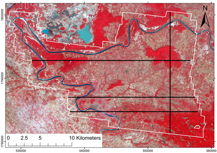
Fig. 1. False-color ALOS AVNIR image of the area. Black transects indicate the location of simulated lidar strips that were used to train the models. The area with lidar coverage is outlined in white.
The training data consisted of three east-west strips and one north-south strip (Fig. 1). The strips had 395, 310, 310, and 301 population units, giving a total of 1316 units. The digital numbers of blue, green, red and near infrared bands were extracted for each population unit. The mean and standard deviation of the digital numbers within each 30 × 30 m population unit were also calculated for each band. Band-wise means were used to further calculate different vegetation indices.
The vegetation indices that we tested were simple ratio (SR), normalized difference vegetation index (NDVI), and the atmospherically resistant vegetation index (ARVI). SR and NDVI indices utilize red (RED) and near-infrared (NIR) bands, with the main difference that unlike SR, NDVI is not affected by absolute pixel values (Mather and Koch 2011). The ARVI index also includes the blue band (BLUE), in an attempt to reduce the influence of atmospheric scattering (Kaufman and Tanre 1996). These vegetation indices were calculated as shown in equations 1–3.
2.3 Airborne lidar data
Wall-to-wall lidar data was acquired from the study area on the 6th–8th February 2009. The Leica ALS 40 scanner was flown at a height of 2000 meters to acquire data with a nominal pulse density of 1 / m2. The sidelap between the flight lines was 20%, and maximum scan angle was set at 15°. The scanner was capable of recording up to four echoes per pulse. A Digital Terrain Model (DTM) was created with TerraScan software (TerraSolid 2015) using last and single echoes. The CC was estimated for every 30 × 30 m population unit within the scanned area as the fraction of first and single canopy echoes. This variable is known as the first echo cover index (FCI) (Korhonen et al. 2011):

Echoes > 2.0 m above ground level are considered to represent the canopy.
Ideally the FCIs should be calibrated with field measurements that are compatible with the CC definitions (Jennings et al. 1999; Gschwantner et al. 2009). Unfortunately, reliable calibration data were not available and hence our CC estimates are slightly biased. The FCI is usually slightly larger than the CC which is obtained from sighting tubes, because the ALS pulses are not exactly vertical and therefore have a slightly larger probability of hitting the crowns than vertical pulses. The bias caused by this effect was between 1–5% when the scan zenith angle was less than 15° (Korhonen et al. 2011). In addition, some of the tree species in the dry dipterocarp forests were leafless, and thus it is likely that the CC was underestimated in these forests, although the correlation has also been shown to be strong in a leaf-off situation (Parent and Volin 2014). Thus both the real and estimated CCs are different in the dry and wet seasons. The dry season is however the best option for lidar and optical image data acquisition because of the persistent cloud cover which is present during the wet season. Nevertheless, the FCI reliably describes the whole range of CC variations which occur in the area.
The 30 × 30 m population units obtained from the strips and used for training the model are from this point onwards, termed as lidar plots. For the rest of the study, we use the acronym “FCI” when discussing CC estimates obtained specifically from the lidar data. “CC” is used when referring to the canopy cover in general. Fig. 2 displays a histogram of the FCI values within the lidar plots. The indigenous mixed deciduous forests with an FCI > 90% are shown as a peak in the histogram, but the majority of the study area is dry dipterocarp forest, or disturbed forest with lower FCI values. Some of the lidar plots also had an FCI = 0% (n = 12) or 100% (n = 13).
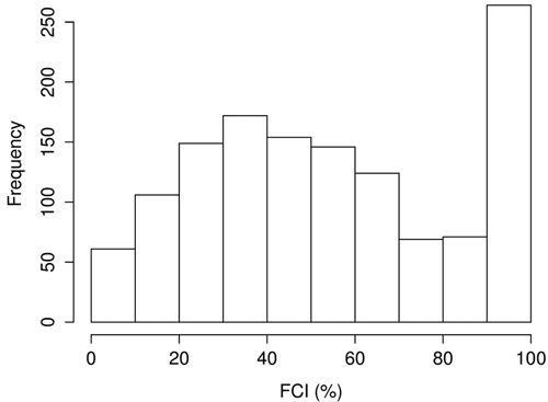
Fig. 2. Histogram of the first echo cover index (FCI) values within our data set.
2.4 Statistical methods
Linear regression analysis is not well suited for the estimation of CC, because the predictions must be restricted to the 0–1 interval. Beta regression (Ferrari and Cribari-Neto 2004) presents a better alternative for CC estimation (Korhonen et al. 2007; Coulston et al. 2012) as the response variable is assumed to be a sample from a beta distribution with unknown parameters. The mean and dispersion parameters of the distribution are estimated based on the sample so that the mean parameter is related to the predictor variables by a regression structure, while the dispersion parameter is assumed to be constant. Beta regression also enables the selection of a link function that keeps the predictions in the correct range. However, it is not capable of dealing with lidar plots having a 0% or 100% cover, because the beta distribution is not defined for these values. Both extremes were present in our data, and therefore we applied zero-and-one inflated beta regression (ZOINBR) which is capable of solving this issue. Alternatively, it would have been possible to use nonparametric regression methods such as the K-most similar neighbor (Moeur and Stage 1995). We tested K-MSN against ZOINBR and found that the prediction accuracy was slightly weaker, so in this study, only the ZOINBR results are reported.
Zero-and-one inflated beta distribution is an extension to the beta distribution that can be used to model percent data that contains ones and zeroes (Ospina and Ferrari 2010). ZOINBR models can be fitted using the R statistical software (R core team 2012) and the external library gamlss (Stasinopoulos and Rigby 2007). Gamlss (generalized additive models for location, scale and shape) is meant to overcome the limitations of generalized linear and additive models. The response variable is assumed to follow a parametric distribution, but it does not need to belong to the exponential family and can be either skewed, kurtotic or discrete.
The gamlss models assume that independent observations yi with a probability density function f(yi|θ) are conditional on the vector θ = (μi, σi, νi, τi) with four distribution parameters, each of which can be a function of the explanatory variables (Stasinopoulos and Rigby 2007). Parameters μi and σi are typically related to the location and scale of the distribution, while νi and τi represent the skewness and kurtosis. However, the model can also be applied for distributions with different parameters, and the parameters can be estimated as linear, nonlinear, or a smooth function of the explanatory variables.
The zero-and-one inflated beta distribution is a mixture distribution that combines beta and Bernoulli distributions so that probability mass can also be allocated for the values 0and 1. The beta distribution has several parameterizations. The one used in gamlss has the location parameter μ and the scale parameter σ, and its probability density function for 0< y < 1 is as follows (Stasinopoulos et al. 2008):

where B is the beta function, α = μ (1–σ2)/σ2, β = (1–μ) (1- σ2)/ σ2, α > 0and β > 0. The zero-and-one inflated beta distribution extends this function by introducing additional parameters p0 and p1, which describe probabilities that the observed value is 0or 1, respectively. The probability density function is written as:

for 0 ≤ y ≤ 1, where α and β are as above, p0 = ν (1+ν+τ)–1, p1 = τ (1+ ν+τ)–1, α > 0, β > 0, 0 ≤ p0 ≤ 1, and 0 ≤ p1 ≤ 1 (Stasinopoulos et al. 2008). The parameters μ, σ, ν, and τ are estimated using the method of maximum (penalized) likelihood. Monotonic link functions that can be defined separately for each variable are used in the process. By default, the link functions are logistic, logistic, log and log for μ, σ, ν, and τ, respectively. The final parameter estimates are calculated from the values given by the gamlss by applying an inverse of the link function. The expected value of the distribution (μ) is dependent on the predictor variables as defined by the estimated regression coefficients. Using the logistic link function, μ is modelled as:

where βj = the vector of model coefficients and xj = the vector of predictor variables. The estimate for μ (which is also the model prediction) is obtained by applying the inverse of the logistic function:
Variable selection for the ZOINBR models was based on an exhaustive search to find the two and three-variable combinations having the lowest model RMSE of predictions:

where yi = FCI, ŷi = the estimate derived from the satellite images, and n = the number of lidar plots. The most promising predictors and their transformations were tested manually to find the model having the best RMSE in leave-strip-out cross validation (LSO-CV). Each of the four strips with 301–395 lidar plots per strip was omitted from the data one at a time, and the remaining lidar plots were used to fit the model. The model was then applied to predict the FCI of the lidar plots in the omitted strip, and the RMSE and bias (Eq. 10) were calculated for the predictions.

We report all RMSE and bias values as percent points, i.e. they are absolute values that describe the difference between the observed and predicted values (not divided by the mean of response variable). In order to enable a comparison with earlier studies, we also calculated the pseudo-R2 as a square of the sample correlation coefficient between the values estimated in the LSO-CV and the observed values (Ferrari and Cribari-Neto 2004).
2.5 Forest – non-forest classification
We tested the binary classification of lidar plots into either forest or non-forest, based on the CC. We tested both the international (10%) and the national (20%) CC limits, but as the differences in model accuracy were small, only the results obtained using the 20% limit are reported. In addition, we compared the direct and indirect estimations of the forest area. In the direct estimation, we converted the lidar-based FCI values into forest or non-forest based on the 20% FCI limit, and the new binary variable was used as a response in the resulting classification. In the indirect estimation, the FCIs were first predicted and then converted into forest or non-forest.
Because the response variable was binary (1 = forest, 0= non-forest), logistic regression was employed instead of the ZOINBR. Logistic regression models are generalized linear models, where the response variable is assumed to follow a Bernoulli distribution. A logistic link function (Eq. 7) was applied in all cases. Variable selection was similar to ZOINBR, but Cohen’s kappa coefficient (Landis and Koch 1977) was used as the main criterion. Overall, the user’s and producer’s accuracies were also calculated from the error matrices.
2.6 Map comparisons
The satellite-based models were applied to create maps of FCI and forest area, and validated against the wall-to-wall FCI map. A water mask was applied to exclude the population units that included water bodies. Settlement areas were also excluded because the lidar echoes from buildings could be erroneously interpreted as canopy echoes. The rest of the land area (n = 409 217 population units) was included in the comparisons, regardless of the land use. In addition to maps showing the estimated and observed FCI and FCI-based forest area, we created maps that visualized the magnitude of error in satellite-based FCI predictions and the types of error in the direct forest/non-forest classification. Aerial photographs were utilized to visually inspect those sites with considerable errors. RMSE, bias, and the pseudo-R2 of the FCI were also calculated for the entire population, as well as the kappa coefficient and error matrix of the forest/non-forest classification.
3 Results
3.1 Canopy cover
The coefficients of our final zero-and-one inflated beta regression model of the training data are displayed in Table 1. The model shape is quadratic polynomial with two predictor variables: the vegetation index ARVI and the blue band digital number. In the LSO-CV, the model’s absolute RMSE was 11.5% and the pseudo R2 was 0.85. The μ parameter was related to the predictors through regression structure and logistic link function, while the other parameters were constant. Differences in RMSE among the different variable combinations were fairly small, with most producing RMSEs of 12–13% in the LSO-CV.
| Table 1. Zero-and-one inflated beta regression model for the estimation of canopy cover. All coefficients were statistically significant with P < 10–10. The model deviance was –2260.1 and the AIC (Akaike Information Criterion) was –2244.1. | ||||
| Parameter | Link function | Variable | Coefficient | Standard error |
| μ | Logit | Intercept | –48.32 | 3.91 |
| ARVI | 4.139 | 0.202 | ||
| ARVI2 | 1.148 | 0.182 | ||
| BLUE | 0.9399 | 0.0792 | ||
| BLUE2 | –0.004635 | 0.000401 | ||
| σ | Logit | Intercept | –0.9962 | 0.0232 |
| ν | Log | Intercept | –4.678 | 0.290 |
| τ | Log | Intercept | –4.598 | 0.0279 |
Fig. 3 shows a scatter diagram where the estimates obtained from the ALOS image by applying ZOINBR and LSO-CV are plotted against the FCIs obtained from the lidar data. Lidar plots with an FCI close to 100% usually had an estimated FCI ranging from 85% to 100%, and as these cases were common in our data, they seem to be the main reason for the slight overall underestimation as indicated by the measured bias (0.6%). Underestimation of lidar plots with a very high FCI could not be totally avoided, but in practical applications, FCI estimates ranging from 90% to 100% would have a similar interpretation. The opposite occurred at the lower end of the scale, where the FCI was overestimated by up to 20% in lidar plots with an observed FCI close to zero. Although the number of these cases was fairly low, they could be important because such errors influence the forest/non-forest classification. In the middle of the FCI range, the model fitted the data well, but individual errors in the estimated FCI could be as high as 30%.
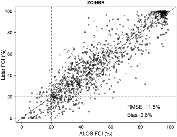
Fig. 3. The relationship between lidar-based canopy cover estimates (FCI) and estimates obtained from the satellite image using zero-and-one inflated beta regression (ZOINBR). Dashed lines show the 20% FCI threshold used in forest/non-forest classification.
Including the blue band as a predictor improved the model performance, especially at the lower end of the FCI scale. When the blue band was removed or replaced by the NIR band, the model never predicted FCIs smaller than 15%. Green and red bands had a high correlation with the blue band (R = 0.97 and 0.95 respectively), and using these instead of the blue band also improved the model, but not as much (RMSE = 11.9% and 11.7% respectively). The ARVI index performed better than the NDVI and SR, both of which provided an RMSE of 12.7% when applied instead of the ARVI index and using the same model shape. The two-predictor models that included the ARVI index always provided smaller RMSEs than models without it (the smallest RMSE being 11.5% vs. 12.5% respectively).
The FCI map obtained using the model shown in Table 1 and its error map are shown as figures 4 and 5. The model RMSE in the entire population was 12.8%, bias 0.55%, and the pseudo-R2 was 0.82, i.e. the accuracy was slightly worse than the estimates obtained from LSO-CV indicated. The error map indicated that inclusion of other land use categories within the scanned area was one of the main sources of error. For example, a troublesome area around the river bend in the north-west region of the map (Fig. 5) included agricultural areas where the FCI was overestimated. In addition, this area had bamboo thickets where the vegetation was so dense that no last echoes were received from the ground, and the DTM was estimated to follow the surface of the bamboo. Thus, the spectral FCI estimates for such sites were close to 100%, while the lidar-based FCIs were close to zero.
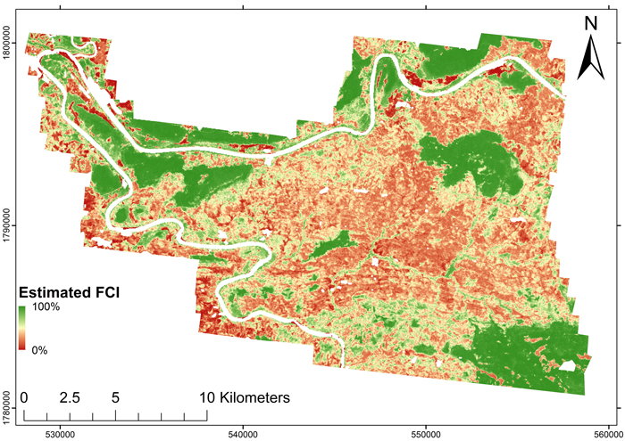
Fig. 4. First echo cover index (FCI) map obtained from the ALOS AVNIR-2 image for the area with lidar coverage.
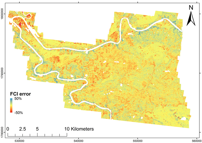
Fig. 5. Error map of the estimated first echo cover index (FCI) obtained from comparison with a lidar-based map. The FCI was underestimated in the blue areas and overestimated in the red areas.
Forest areas with underestimation problems included trees with low near-infrared reflectance, i.e. leafless dipterocarps whose crowns were still captured by the lidar. These forests were also represented in the modelling data set, but the model was unable to adequately fit both the evergreen mixed deciduous and dry dipterocarp forests, and which probably explains a large proportion of the residual variance. FCI was also somewhat overestimated in areas where the forest was cleared for slash-and-burn cultivation or for some other land use. This could have been caused by the relatively small number of low-FCI stands in our training data (Fig. 2), which probably resulted in a tendency to overestimate stands with a low FCI. This can also be observed in Fig. 3 where a majority of lidar plots with an observed FCI of < 20% are actually predicted to have an FCI > 20%.
3.2 Forest and non-forest
Our best logistic model for the direct prediction of forest area, and employing quadratic polynomials of the vegetation indices ARVI and NDVI as predictors is shown below:

where µ is the expected value of the predicted Bernoulli distribution.
The model AIC was 529.1 and the residual deviance was 519.1 on 1311 degrees of freedom. The model’s kappa coefficient was 0.60 and its overall accuracy was 91.0%. This result was superior to indirect estimation where the FCIs predicted by the ZOINBR model (Table 1) were converted to forest or non-forest. The indirect estimation only achieved a kappa = 0.45 in the LSO-CV, although the overall accuracy was equally as good (90.4%). Error matrices obtained from the LSO-CV are shown in Table 2 for both methods. The indirect estimation with the ZOINBR model produced a very high producer’s accuracy for forest (98.2%), which had more observations than the non-forest class (1149 vs. 167). Thus, the indirect estimation’s low producer accuracy for non-forest (37.1%) is only reflected in the kappa coefficient (0.45). The reason for this could be that a majority of the lidar plots had high FCI values, and optimizing the ZOINBR model for FCI weighted the densely covered lidar plots more than the smaller number of low FCI plots.
| Table 2. Error matrices of the indirect (ZOINBR) and direct (logistic model) forest/non-forest classification using a 20% FCI threshold in the leave-strip-out cross validation. Kappa coefficients were 0.45 and 0.60 respectively. | |||||
| Observed | User’s accuracy | ||||
| Predicted | Method | Non-forest | Forest | Sum | |
| Non-forest | ZOINBR | 62 | 21 | 83 | 74.7% |
| Logistic model | 110 | 62 | 172 | 64.0% | |
| Forest | ZOINBR | 105 | 1128 | 1233 | 91.5% |
| Logistic model | 57 | 1087 | 1144 | 95.0% | |
| Sum | 167 | 1149 | 1316 | ||
| Producer’s | ZOINBR | 37.1% | 98.2% | 90.4% | |
| Logistic model | 65.9% | 94.6% | 91.0% | ||
The error matrices of direct and indirect forest area estimation for the whole area are shown in Table 3. The direct model’s kappa coefficient in this classification was 0.61 and the overall accuracy was 90.6%, i.e. very close to the values obtained in the leave-strip-out cross validation. For the indirect approach, the kappa coefficient was 0.53, i.e. better than shown in the LSO-CV. Based solely on the CC criterion, the logistic model prediction for forest coverage within the area was 87.9%, while the lidar-based observed value was 84.5%, i.e. the forest area was slightly overestimated. Table 3 shows that non-forest was more difficult to classify correctly than forest (user’s accuracy 75.4% vs. 92.7%). The producer’s accuracy for non-forest was only 58.7%, indicating that 41.3% of the observed non-forest area was misclassified as forest. Again, the main reason for this could be the insufficient number of low FCI plots contained in the training data.
| Table 3. Error matrices of the indirect (ZOINBR) and direct (logistic model) forest/non-forest classification using a 20% FCI threshold for the whole population. Kappa coefficients were 0.53 and 0.61 respectively. | |||||
| Observed | User’s accuracy | ||||
| Predicted | Method | Non-forest | Forest | Sum | |
| Non-forest | ZOINBR | 28 500 | 5 645 | 34 145 | 83.5% |
| Logistic model | 37 330 | 12 171 | 49 501 | 75.4% | |
| Forest | ZOINBR | 35 095 | 339 977 | 375 072 | 90.6% |
| Logistic model | 26 265 | 333 451 | 359 716 | 92.7% | |
| Sum | 63 595 | 345 622 | 409 217 | ||
| Producer’s | ZOINBR | 44.8% | 98.3% | 90.0% | |
| Logistic model | 58.7% | 96.5% | 90.6% | ||
The error map of the direct forest/non-forest classification is shown as Fig. 6, and the lidar-based map of the non-forest areas is shown as Fig. 7. Visual inspection of the error map showed that the indigenous, high-cover forests were consistently classified correctly. Erroneous pixels were scattered all around the map, but the majority occurred within the disturbed forest area which featured in the middle of the mapped area, where non-forest areas were frequently classified as forest. The non-forest pixels classified as forest occurred typically in areas which were cleared for agriculture as visualized in Fig. 8. The paddy fields were without vegetation during the dry season and therefore usually classified correctly, but already, a few pixels with a high near-infrared reflectance could cause the population unit to be classified as forest (Fig. 8). Classifying forest as non-forest occurred less frequently, and mostly in the dry dipterocarp forests with a fairly low near-infrared reflectance.
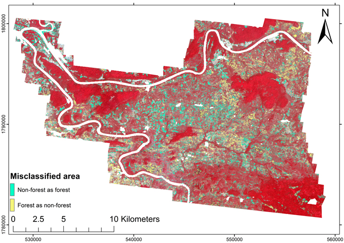
Fig. 6. Error map of the forest/non-forest classification using the logistic model (Eq. 11).
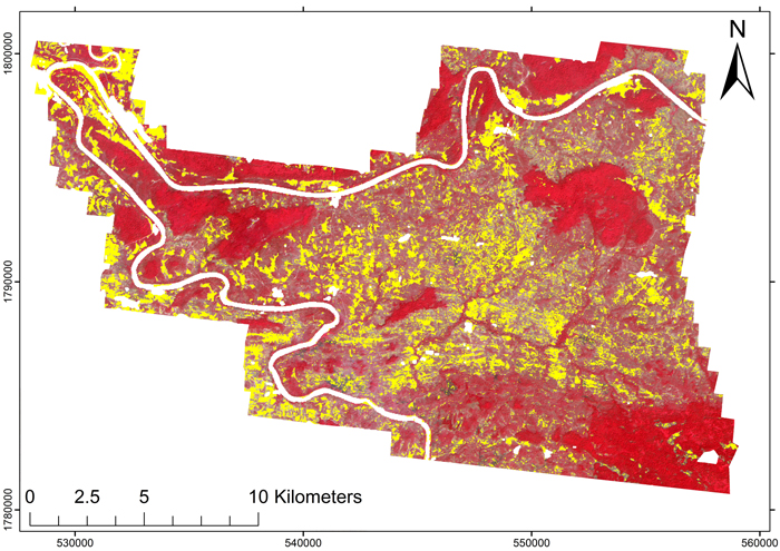
Fig. 7. Lidar-based map of the non-forest areas (yellow). Based on the lidar, 84.5% of the scanned area was forest, based on the 20% FCI criterion. Also, the areas between the indigenous mixed deciduous forests frequently had an FCI > 20%.
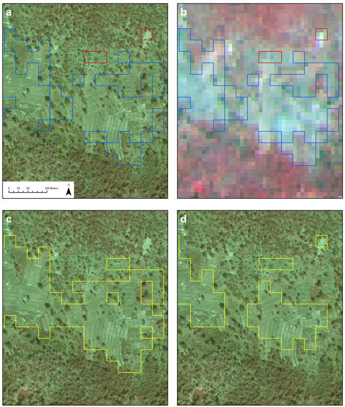
Fig. 8. Typical site with classification errors. Panel a) shows the classification errors visualized in an aerial image, and b) in the ALOS AVNIR-2 satellite image. Blue polygons are non-forest areas classified as forest, red polygons forest areas classified as non-forest. Below, c) shows the extent of the lidar-based non-forest area, and d) its ALOS-based estimate upon the aerial image. View larger in new window/tab.
4 Discussion
Our attempt to estimate lidar-based canopy cover using an ALOS AVNIR-2 image performed well, as our pseudo-R2 values (full population = 0.82, cross validated = 0.85) are high compared to earlier studies (e.g. Carreiras et al. 2006; Wolter et al. 2009), and especially encouraging for estimating the tropical forests of south-east Asia (Koy et al. 2005). We assume that the high consistency of the lidar-based FCI proxy for CC helped to achieve this result, because commonly applied quick field-based CC estimates or estimates derived from the visual interpretation of higher resolution optical images are less accurate than lidar-based FCIs. When the uncertainty of the estimated CC is small, a major source of error is removed from the modelling. Lidar data can also be intersected exactly for the selected satellite pixels, which decreases the scale mismatch between validation data and satellite imagery. However, our study area was fairly small, which probably contributed to the high degree of accuracy due to the small amounts of atmospheric variation within the area of interest. Therefore we could utilize the blue band that is otherwise prone to atmospheric variations (Häme et al. 2013).
Although the lidar-based CC estimates are slightly biased, in visual interpretation, the lidar-based forest area map showed a very good agreement with the aerial images (Fig. 8). It is recommended to measure a small number of reference plots (e.g. 10–20) with a sighting tube so that the range of CC within the inventory area is covered, and then to calibrate the FCIs with these values. If the field data is lacking, the FCIs can still provide a meaningful description of the CC gradients within the area. Future work should therefore focus on understanding the scanner settings, so that the biases caused by non-vertical scanning could be corrected using empirical models if calibration data is not available.
The ZOINBR is well suited for large-area CC estimation because the predictions are guaranteed to remain logical and plots with 0% or 100% CCs are allowed. The only noticeable problem with the ZOINBR method was the slight underestimation in stands with a nearly 100% FCI, but in practice, all forests with a CC close to 100% can be considered to be undisturbed. The other sources of error observed in the prediction were not related to the modelling technique. The reasons for these errors were usually either the application of the model in population units without trees or mixed land uses, or an inadequate number of lidar plots with FCIs < 20% (12.7%) in the training data, which resulted in a poor level of accuracy in areas with a low CC. Also, defoliation of the dry dipterocarp forests had a noticeable influence. A forest area mask can also be estimated from the same data using the logistic regression shown above. In our initial test in Finland, the RMSE of the FCI model increased by six percentage points when it was applied to systematically placed validation plots (Korhonen et al. 2013).
In the forest/non-forest classification, the direct logistic model provided better results than when first estimating the CC and then classifying the estimated values, because it was optimized to separate those lidar plots close to the FCI threshold. It is also possible to use the CC models for forest classification, but this criterion should also be included in the variable selection. The balance of the data set would be more of an issue if the international 10% CC limit was applied instead of the local 20% limit, because the number of observations needed in the modelling increases with unequal class sizes.
Our study focused on the pixel scale mapping of CC and forest/non-forest classification, based solely on the CC criterion. In practical forest cover mapping, other criteria mentioned in the international definition for forests must also be included (FAO 2005), including minimum area, minimum width, tree height and land use. Thus, in further applications the full processing chain described by Magdon et al. (2014) should be followed. In practical scenarios, field measurements of both CC and height are needed to obtain unbiased estimates. We also used a fixed size for the population unit, although this can influence the results of forest area estimation (Eysn et al. 2012). In addition, we did not filter the 30-m resolution maps for noise pixels or generalize them into a smaller resolution, both of which should be done for practical map products.
Our results concerning forest area are somewhat different from those of Häme et al. (2013), who used the same ALOS AVNIR-2 data set to create a mosaicked land cover map for the whole province of Savannakhet. They used high-resolution Quickbird and Kompsat images to visually interpret the land use for spectrally similar classes obtained from unsupervised fuzzy classification, and then applied the classification to create large-area maps. Looking at this land use map (Häme et al. 2013, Fig. 7, N = 1 790 000, E = 550 000), our study area is mostly classified as farmland, cleared forest, or other non-forest. Their results are not directly comparable to ours, as we focused solely on the CC criterion and ignored the influence of land use. Nevertheless, based on our lidar-derived FCI map (Fig. 7), the CC was also commonly above 20% in areas where a visual interpretation may indicate other land use. Also, our observed forest percentage (84.5%) seems considerably higher than the map by Häme et al. (2013) would indicate.
In the case of a large-scale inventory, several images are needed to cover the area of interest. In such cases the lidar strips should be placed so that a sufficient number of lidar plots are available within each image, so as to avoid the need to apply models to images without reference data. Forest area maps should also be supplemented by confidence intervals for the variables of interest, and these can be obtained e.g. by the application of model-based or model-assisted sampling equations (McRoberts et al. 2014). In our study, the placement of the lidar strips used for training the model was subjective, which corresponds to an inventory with a model-based approach. With the model-based approach, the main objective of the training data collection is to maximize the model validity by selecting the training data to be as diverse as possible. The selection of strip samples should therefore be planned carefully, so that sufficient samples are obtained from all forest types within the area of interest.
Acknowledgements
The authors thank the SUFORD project and the Finnish Ministry of Foreign Affairs for their support for the data acquisition. Arbonaut Oy Ltd. kindly provided the data sets from Lao PDR. The study was funded by the strategic funds of the University of Eastern Finland (spearhead project “Multi-scale geospatial analysis of forest ecosystems”) and the Academy of Finland (grant no. 252257).
References
Achard F., Beuchle R., Mayaux P., Stibig H.J., Bodart C., Brink A., Carboni S., Desclée B., Donnay F., Eva H.D., Lupi A., Raši R., Seliger R., Simonetti D. (2014). Determination of tropical deforestation rates and related carbon losses from 1990 to 2010. Global Change Biology 20(8): 1365–2486. http://dx.doi.org/10.1111/gcb.12605.
Andersen, H-E., Strunk J., Temesgen H., Atwood T., Winterberger G. (2011). Using multilevel remote sensing and ground data to estimate forest biomass resources. Canadian Journal of Remote Sensing 37: 596–611. http://dx.doi.org/10.5589/m12-003.
Asner G.P., Powell G.V.N., Mascaro J., Knapp D.E., Clark J.K., Jacobson J., Kennedy-Bowdoin T., Balaji A., Paez-Acosta G., Victoria E., Secada L., Valqui M., Hughes R.F. (2010). High-resolution forest carbon stocks and emissions in the Amazon. Proceedings of the National Academy of Sciences 107 (38): 16738–16742. http://dx.doi.org/10.1073/pnas.1004875107.
Carreiras J.M.B., Pereira J.M.C., Pereira J.S. (2006). Estimation of tree canopy cover in evergreen oak woodlands using remote sensing. Forest Ecology and Management 223(1–3): 45–53. http://dx.doi.org/ 10.1016/j.foreco.2005.10.056.
Coulston J.W., Moisen G.G., Wilson B.T., Finco M.V., Cohen W.B., Brewer C.K. (2012). Modeling percent tree canopy cover: a pilot study. Photogrammetric Engineering & Remote Sensing 78(7): 715–727. http://dx.doi.org/10.14358/PERS.78.7.715.
Eysn L., Hollaus M., Schadauer K., Pfeifer N. (2012). Forest delineation based on airborne LIDAR data. Remote Sensing 4: 762–783. http://dx.doi.org/10.3390/rs4030762.
FAO (2005). Global Forest Resources Assessment 2005. Food and Agriculture Organization of the United Nations, Forestry Paper 147. Rome, Italy. 350 p. http://www.fao.org/docrep/008/a0400e/a0400e00.htm. [Cited 16 July 2015].
Ferrari S.L.P., Cribari-Neto F. (2004). Beta regression modeling rates and proportions. Journal of Applied Statistics 31(7): 799–815. http://dx.doi.org/10.1080/0266476042000214501.
Franklin S.E., Hall R.J., Smith L., Gerylo G.R. (2003). Discrimination of conifer height, age and crown closure classes using Landsat-5 TM imagery in the Canadian Northwest Territories. International Journal of Remote Sensing 24(9): 1823–1834. http://dx.doi.org/10.1080/01431160210144589.
Gatziolis D. (2012). Comparison of lidar- and photointerpretation-based estimates of canopy cover. In: McWilliams W, Roesch FA (eds.). Monitoring across borders: 2010 joint meeting of the Forest Inventory and Analysis (FIA) Symposium and the Southern Mensurationists. e-Gen. Technical report SRS-157. U.S. Department of Agriculture, Forest Service, Southern Research Station, Asheville, NC. p 231–235. http://www.treesearch.fs.fed.us/pubs/41012. [Cited 16 July 2015].
Gemmell F., Varjo J., Strandström M. (2001). Estimating forest cover in a boreal forest test site using thematic mapper data from two dates. Remote Sensing of Environment 77: 197–211. http://dx.doi.org/10.1016/S0034-4257(01)00206-1.
Gschwantner T., Schadauer K., Vidal C., Lanz A., Tomppo E., di Cosmo L., Robert N., Duursma D.E., Lawrence M. (2009). Common tree definitions for national forest inventories in Europe. Silva Fennica 43(2): 303–321. http://dx.doi.org/10.14214/sf.463.
Häme T., Kilpi J., Ahola H.A., Rauste Y., Antropov O., Rautiainen M., Sirro L., Bounpone S. (2013). Improved mapping of tropical forests with optical and SAR imagery, part I: forest cover and accuracy assessment using multi-resolution data. IEEE Journal of Selected Topics in Applied Earth Observations and Remote Sensing 6(1): 74–91. http://dx.doi.org/10.1109/jstars.2013.2241019.
Jennings S.B., Brown N.D., Sheil D. ( 1999). Assessing forest canopies and understory illumination: canopy closure, canopy cover and other measures. Forestry 72(1): 59–74. http://dx.doi.org/10.1093/forestry/72.1.59.
Kaufman Y.J., Tanre D. (1996). Strategy for direct and indirect methods for correcting the aerosol effect on remote sensing: from AVHRR to EOS-MODIS. Remote Sensing of Environment 55(1): 65–79. http://dx.doi.org/10.1016/0034-4257(95)00193-X.
Korhonen L., Korhonen K.T., Rautiainen M., Stenberg P. (2006). Estimation of forest canopy cover: a comparison of field measurement techniques. Silva Fennica 40(4): 577–588. http://dx.doi.org/10.14214/sf.315.
Korhonen L., Korhonen K.T., Stenberg P., Maltamo M., Rautiainen M. (2007). Local models for forest canopy cover with beta regression. Silva Fennica 41(4): 671–685. http://dx.doi.org/10.14214/sf.275.
Korhonen L., Korpela I., Heiskanen J., Maltamo M. (2011). Airborne discrete-return LIDAR data in the estimation of vertical canopy cover, angular canopy closure and leaf area index. Remote Sensing of Environment 115: 1065–1080. http://dx.doi.org/10.1016/j.rse.2010.12.011.
Korhonen L., Heiskanen J., Korpela I. (2013). Modelling lidar-derived boreal forest canopy cover with SPOT 4 HRVIR data. International Journal of Remote Sensing 34(22): 8172–8181. http://dx.doi.org/10.1080/01431161.2013.833361.
Koy K., McShea W.J., Leimgruber P., Haack B.N., Aung M. (2005). Percentage canopy cover – using Landsat imagery to delineate habitat for Myanmar’s endangered Eld’s deer (Cervus eldi). Animal Conservation 8: 289–296. http://dx.doi.org/10.1017/S1367943005002209.
Landis R.J., Koch G.G. (1977). The measurement of observer agreement for categorical data. Biometrics 33: 159–174.
Magdon P., Fischer C., Fuchs H., Kleinn C. (2014). Translating criteria of international forest definitions into remote sensing image analysis. Remote Sensing of Environment 149: 252–262. http://dx.doi.org/10.1016/j.rse.2014.03.033.
Mather P.M., Koch M. (2011). Computer processing of remotely-sensed images: an introduction, fourth edition. John Wiley & Sons, Inc. 462 p. http://dx.doi.org/10.1002/9780470666517.
McRoberts R.E., Næsset E., Gobakken T. (2014). Estimation of inaccessible and non-sampled forest areas using model-based inference and remotely sensed auxiliary information. Remote Sensing of Environment 154: 226–233. http://dx.doi.org/10.1016/j.rse.2014.08.028.
Moeur M., Stage A.R. (1995). Most similar neighbor: an improved sampling inference procedure for natural resource planning. Forest Science 41(2): 337–359.
Ospina R., Ferrari S.L.P. (2010). Inflated beta distributions. Statistical Papers 51(1): 111–126. http://dx.doi.org/10.1007/s00362-008-0125-4.
Parent J.R., Volin J.C. (2014). Assessing the potential for leaf-off LiDAR data to model canopy closure in temperate deciduous forests. ISPRS Journal of Photogrammetry and Remote Sensing 95: 134–145. http://dx.doi.org/10.1016/j.isprsjprs.2014.06.009.
R Core Team (2012). R: a language and environment for statistical computing. R Foundation for Statistical Computing, Vienna, Austria. ISBN 3-900051-07-0. http://www.R-project.org/. [Cited 16 July 2015].
Sexton J.O., Song X.P., Feng M., Noojipady P., Anand A., Huang C., Kim D.H., Collins K.M., Channan S., DiMiceli C. Townshend J.R. (2013). Global, 30-m resolution continuous fields of tree cover: Landsat-based rescaling of MODIS vegetation continuous fields with lidar-based estimates of error. International Journal of Digital Earth 6(5): 427–448. http://dx.doi.org/10.1080/17538947.2013.786146.
Song C., Woodcock C.E., Seto K.C., Lenney M.P., Macomber S.A. (2001). Classification and change detection using Landsat TM data: when and how to correct atmospheric effects? Remote Sensing of Environment 75: 230–244. http://dx.doi.org/10.1016/S0034-4257(00)00169-3.
Stasinopoulos D.M., Rigby R.A. (2007). Generalized additive models for location, scale and shape (GAMLSS) in R. Journal of Statistical Software 23(7): 1–46. http://www.jstatsoft.org/v23/i07/paper. [Cited 16.7.2015].
Stasinopoulos M., Rigby B., Akantziliotou C. (2008). Instructions on how to use the gamlss package in R, Second edition. Available at: http://www.gamlss.org/wp-content/uploads/2013/01/gamlss-manual.pdf. [Cited 9 June 2015].
Stojanova D., Panov P., Gjorkioski V., Kobler A., Džeroski S. (2010). Estimating vegetation height and canopy cover from remotely sensed data with machine learning. Ecological Informatics 5: 256–266. http://dx.doi.org/10.1016/j.ecoinf.2010.03.004.
Strunk J.L., Temesgen H., Andersen H.E., Packalen P. (2014). Prediction of forest attributes with field plots, Landsat, and a sample of lidar strips: a case study on the Kenai peninsula, Alaska. Photogrammetric Engineering & Remote Sensing 80(2): 143–150. http://dx.doi.org/10.14358/PERS.80.2.143.
Terrasolid (2015). Terrasolid - the standard for airborne and mobile LiDAR and image processing. http://www.terrasolid.fi/en. [Cited 9 June 2015].
United Nations Framework Convention on Climate Change (UNFCCC) (2001). Report of the Conference of the Parties on its seventh session (COP7), Part two: action taken by the Conference of the Parties. Marrakesh, Morocco. 69 p.
Wolter P.T., Townsend P.A. Sturtevant B.R. (2009). Estimation of forest structural parameters using 5 and 10 meter SPOT-5 satellite data. Remote Sensing of Environment 113: 2019–2036. http://dx.doi.org/10.1016/j.rse.2009.05.009.
Total of 37 references
Send to email

