Ilya Potapov  ,
Marko Järvenpää,
Markku Åkerblom,
Pasi Raumonen,
Mikko Kaasalainen
,
Marko Järvenpää,
Markku Åkerblom,
Pasi Raumonen,
Mikko Kaasalainen
Data-based stochastic modeling of tree growth and structure formation
Potapov I., Järvenpää M., Åkerblom M., Raumonen P., Kaasalainen M. (2015). Data-based stochastic modeling of tree growth and structure formation. Silva Fennica vol. 50 no. 1 article id 1413. https://doi.org/10.14214/sf.1413
Highlights
- We propose a stochastic version of the tree growth model LIGNUM for producing tree structures consistent with detailed terrestrial laser scanning data, and we provide the proof-of-concept by using model-based simulations and real laser scanning data
- Trees produced with the data-based model resemble the trees of the dataset, and are statistically similar but not copies of each other
- the number of such synthetic trees is not limited.
Abstract
We introduce a general procedure to match a stochastic functional-structural tree model (here LIGNUM augmented with stochastic rules) with real tree structures depicted by quantitative structure models (QSMs) based on terrestrial laser scanning. The matching is done by iteratively finding the maximum correspondence between the measured tree structure and the stochastic choices of the algorithm. First, we analyze the match to synthetic data (generated by the model itself), where the target values of the parameters to be estimated are known in advance, and show that the algorithm converges properly. We then carry out the procedure on real data obtaining a realistic model. We thus conclude that the proposed stochastic structure model (SSM) approach is a viable solution for formulating realistic plant models based on data and accounting for the stochastic influences.
Keywords
terrestrial lidar;
form diversity;
morphological plasticity;
stochastic functional-structural plant model;
quantitative structure models;
data fitting
-
Potapov,
Tampere University of Technology, Department of Mathematics, P.O. Box 553, FI-33101 Tampere, Finland
E-mail
ilya.potapov@tut.fi
- Järvenpää, Tampere University of Technology, Department of Mathematics, P.O. Box 553, FI-33101 Tampere, Finland E-mail marko.jarvenpaa@tut.fi
- Åkerblom, Tampere University of Technology, Department of Mathematics, P.O. Box 553, FI-33101 Tampere, Finland E-mail markku.akerblom@tut.fi
- Raumonen, Tampere University of Technology, Department of Mathematics, P.O. Box 553, FI-33101 Tampere, Finland E-mail pasi.raumonen@tut.fi
- Kaasalainen, Tampere University of Technology, Department of Mathematics, P.O. Box 553, FI-33101 Tampere, Finland E-mail mikko.kaasalainen@tut.fi
Received 29 June 2015 Accepted 14 October 2015 Published 3 November 2015
Views 85688
Available at https://doi.org/10.14214/sf.1413 | Download PDF

1 Introduction
Readily available algorithms for producing realistic and accurately data-calibrated synthetic tree forms would have numerous applications in botany and ecology. Thus far, studies of tree forms have focused either on data representations, with models used only to reconstruct a particular tree (stand) (Pfeifer et al. 2004; Rutzinger et al. 2011; Raumonen et al. 2013, 2015), or on theoretical models with estimated real conditions used for parameter values (De Reffye et al. 1988; Prusinkiewicz and Lindenmayer, 1990; Weber and Penn 1995; Perttunen et al. 1996). Our aim is to bridge this gap between data and theory. We use a stochastic tree growth model whose structural properties are iteratively fitted to the data to produce tree forms (not limited in number) that are statistically similar to the data tree or trees, but are not copies of each other.
To obtain computationally feasible growth models, we must make a twofold hypothesis in this study. First, we propose that a model can capture the variation of tree forms by a combination of simple deterministic processes and stochastic choices representable by low-dimensional probability distribution functions p. The model can thus reproduce tree shapes even if it is not exactly correct in the biological or probabilistic sense. Second, we assume that tree forms can be represented by sets of low-dimensional spaces with abstract coordinates u in which the occurrence of various geometric features can be depicted, and that the model p can be determined from field-data sets U containing a number of observed u-points when both p and u are well chosen. Note that p operates in the space of model parameters q, whereas u represents the space of observables.
We thus need to create both forward and inverse mappings
Once the former is defined, the latter is obtained by iteratively minimizing a distance measure Ds(Umodel, Udata). The principle of introducing stochastic variation to the parameter values q when the growth of a model is simulated can be applied to virtually any model: recursive (Honda 1971; Prusinkiewicz et al. 2001) or self-organizing (Ulam 1962; Bornhofen and Lattaud 2009); functional (Mäkelä and Hari 1986) or structural (Prusinkiewicz and Lindenmayer 1990; Fisher 1992), or any other.
2 Methods
The overall diagram of the method is depicted in Fig. 1. The main building blocks are: a quantitative structure model (QSM) containing all the geometric and hierarchical information about a tree, a stochastic functional-structural plant model (FSPM), a measure of distance between the structural data of the QSM and FSPM given in some u-spaces, and an optimization algorithm minimizing the distance (e.g., a genetic algorithm). The choices for the technical representations of any of the building blocks are not unique; these, in particular the choice of the distance measure and the u-spaces, will be discussed in greater detail elsewhere.
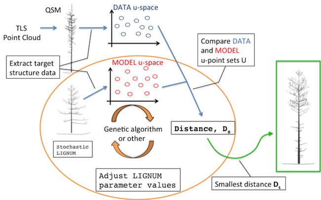
Fig. 1. An overall diagram of the fundamental components of the procedure. The main novelty of this study comprises the orange circle depicting the iterative optimization procedure fitting LIGNUM structural data to those of the field-data Quantitative Structural Model (QSM) that was obtained from the Terrestrial Laser Scanning (TLS) point cloud.
2.1 Data
All structural data can be obtained from a QSM derived from terrestrial laser scanning (TLS) measurements. We used the algorithm described in detail in Raumonen et al. (2013) to extract a QSM from the TLS point cloud data. The field data used here were obtained at a plot of Scots pines in Ruotsinkylä, Finland in 2014 (mean height: 13.2 m, mean breast height diameter: 13.2 cm, stand density: 1932.8 trees·ha–1, total volume: 196.9 m3·ha–1). Results reported here are based on a single QSM derived from the plot.
2.2 Model
As a FSPM to match the data tree structure, we use LIGNUM (Perttunen et al. 1996, 1998, 2001; Lu et al. 2011). Structurally the model consists of cylindrical segments. At each iteration of the model growth, the calculated overall carbon balance (photosynthetic production vs. respiration needs) and the light conditions determine how much biomass is allocated in the consecutive iteration.
The full radiation model implemented in LIGNUM (Perttunen et al. 1998) would be computationally expensive given the large number of iterative simulations necessary in our approach. Therefore, we have modified the radiation model using the shadow propagation method (Palubicki et al. 2009). We divide the space into a grid of voxels each with the associated shadow value S(x,y,z). Each segment is ascribed to a particular voxel creating a pyramidal penumbra at the voxels underneath. Shadow propagation length SL and voxel edge size VS determine, how many voxel layers the shadow propagates down (Table 1; Palubicki et al. 2009). At the top voxel S(x,y,z) = Smax, whereas at the bottom S(x,y,z) = 0(linear interpolation between).
All segments are sequentially processed, producing a 3D grid of accumulated shadow values S(x,y,z). The radiation intercepted by a segment occupying the (x,y,z) voxel is
and the photosynthetic light ratio is
where R is the photosynthetically active radiation in the fully exposed conditions (Table 1). These determine the growth rate (Perttunen et al. 1996, 1998). Also, branches are not allowed to grow further than a radius Renv away from the tree stem, nor intersect other branches or the ground.
| Table 1. The LIGNUM parameters used in this study. Parameters fixed during simulations are reported; the varied (-) and not used (NA) parameters are omitted. Other parameters are from Perttunen et al. (1998) for the synthetic simulation (Section 3.1) and Sievänen et al. (2008) for the real case study (Section 3.2). | |||
| Parameter | Description | Synthetic | Real |
| R | full exposure radiation for a tree segment, relative | 30.0 | 60.0 |
| Smax | maximum shadow induced by a tree segment, relative | 10.0 | - |
| SL | shadow propagation distance, [m] | 0.55 | - |
| VS | linear voxel size, [m] | 0.02 | 0.02 |
| Renv | radius of the circular boundary around the tree stem that the branches are not allowed to cross, [m] | 1.33 | - |
| LR | ratio between the radius and length of a tree segment, dimensionless | - | - |
| Q | apical dominance parameter, varied between 0 (no dominance) and 1 (maximum dominance), dimensionless | - | - |
| βinit , βmax | initial and maximal inclination angles, respectively: angles between the first branch segment and the segment it emanates from, [degree] | - , 95 | - |
| ∆β | inclination angle increment, [degree] | - | - |
| ∆ζ, ∆γ | intensity of the white noise added to the vertical (∆ζ) and horizontal (∆γ) orientations of the segments, [degree] | - , 5 | - |
| T | number of iterations/years of simulation | - | - |
| Tsh | when shedding a branch, the lower age limit for the branch segments | NA | - |
| μsh | parameter to the Poisson variable determining number of the tip segments to shed | NA | - |
Branches with no foliage and no child branches are shed (Sievänen et al. 2008). Since real pine trees contain dead branches, which cannot be effectively distinguished from the live ones in the TLS set-up, we have introduced a delay factor: the youngest segment must be Tsh iterations old for the shedding to occur. Additionally, real trees might have branches shed only partially leaving the dead remnants due to accidental branch break, so we have introduced a Poisson random variable (parameter µsh) determining the number of the tip segments (thinner and thus easier to break than the base) that will be shed while the rest will stay (Table 1).
2.3 Tree form description and model fitting
We determine several quantitative characteristics describing the tree shape, and plot their values as sets U in each chosen abstract plane of coordinates u as shown in Figs. 2 and 3. The variations of the density of the points in u are taken to be the QSM characteristics reflecting the stochastic nature of real tree growth.
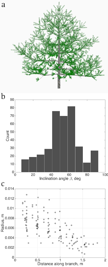
Fig. 2. Sets of points describing the stochastic structure of a tree: a) the simulated LIGNUM tree, source for the data sets; b) the branching/inclination angles of all branches of the 2nd order, (1D set) and c) 1st order tapering, the local cross-section area radius of a branch against the distance from the base of the branch, gathered from all branches of order 1 (2D set). Order is the Gravelius order of a tree such that the lowest order (tree stem) equals to zero.
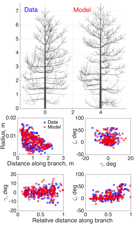
Fig. 3. Model SSM tree shape fitting the emulated QSM “data”, using 8-parameter estimation. Two datasets were used in optimization: 1st order tapering (see also Fig. 2) and spatial curvature, described with two spatial angles (in the horizontal (γ) and vertical (ζ) planes) between consecutive segments as functions of the relative length along branch. The 2D projections of the datasets for the data and the optimized tree are shown in the lower panel.
The original LIGNUM parameters can be changed into and augmented with probability distributions (here simple Gaussian or Poisson ones; see Tables 1 and 2) to catch the stochasticity of growth. As the model tree grows, the effective LIGNUM parameter values q are repeated samples drawn from these distributions p defined by some parameters w.
Using the point plots (Figs. 2 and 3), we compare the characteristic Udata and Umodel of QSM and LIGNUM, respectively. The measure of structural distance Ds[Udata, Umodel (w)] between the two is minimized by adjusting the parameters w, as well as the deterministic LIGNUM parameters, in an iterative optimization procedure (here a genetic algorithm to enable global optimization). The Ds measures the difference between the local densities of the data and model points U in the chosen plot planes. Here its construction is based on Kaasalainen (2008) (cf. Sect. 5 and Eq. (32) therein), but this (or the u-spaces adopted here) is by no means a unique or optimal choice. For example, if we have a large number of u-points from a plot of clones or trees otherwise labeled similar, we can divide the u-space into cells, and minimize the model vs. data difference of the relative density of occupation numbers in each cell.
We call the set of resulting best-fit stochastic FSPM parameters a stochastic structure model (SSM). Note that this is not a fixed tree form: its computer realizations have each time different details but they share a statistically similar appearance.
3 Results
We report two cases, based on the synthetic (generated by stochastic LIGNUM) and real data, respectively. The former demonstrates the possibility of the algorithm to converge to the target tree form and the target parameter values that are known in advance. Additionally, it reveals practical aspects of the algorithm performance and assesses sensitivity of the parameters. Thus, the actual values of the parameters play no significant role in this case.
We opted for the 8-parameter estimation, which was found to be a compromise between the complexity and number of parameters to converge: as the number of parameters grows the possibility of various parametric solutions producing similar tree structures increases. The real data case has no such limitations.
3.1 Model-based synthetic data
As an initial consistency check and a test of our basic modeling principle, we fit the model to simulated QSM data generated by the same model (since the model is stochastic, we do not commit an “inverse crime”; i.e., the optimized SSM tree cannot look exactly like the original one). Here we select eight parameters (Table 2) to be estimated and fix others as in Perttunen et al. (1998). We set the parameter variation ranges for the optimization routine from 50% to 150% of the target value for every parameter, which helps us to assess the parameter estimation accuracy. The coordinates u in which the fitting is depicted are obtained from the branches of the 1st Gravelius order (the stem is of order 0): we choose tapering and spatial curvature of the branches. The former couples the local radius of the branch and the distance from its base. The latter relates the two spatial angles (in horizontal and vertical planes) between the consecutive segments of a branch to the relative distance from its base. The sets U are rendered as scatter plots by considering all branches of the given order. The results are shown in Fig. 3 and Table 2.
| Table 2. Parameter estimation in the emulated “data” case. The tree shapes and fitted structural data sets are shown in Fig. 3. Parameters LR and Q follow the normal distribution having two parameters: mean and standard deviation (std). Other LIGNUM parameters are from Perttunen et al. (1998) and R = 30.0, Smax = 10.0, SL = 0.55 m, VS= 0.02 m, Renv = 1.33 m, βmax = 95 degree, ∆γ = 5 degree, and original shedding options (Sievänen et al. 2008). See Table 1 for the parameter definitions. The genetic algorithm has stopped after 22 full iterations/generations, each generation consisted of 40 parameter sets. | |||
| Parameter name | Data value | Model value (estimated) | Relative error, % |
| LR, mean | 0.009 | 0.0094 | 4.65 |
| LR, std | 0.001 | 0.0009 | 6.95 |
| Q, mean | 0.2 | 0.2058 | 2.88 |
| Q, std | 0.03 | 0.0213 | 28.88 |
| T | 15 | 16 | 6.67 |
| ∆β | 10.0 | 9.7665 | 2.33 |
| ∆ζ | 5.0 | 4.3708 | 12.58 |
| βinit | 35.0 | 40.4649 | 15.61 |
As Fig. 3 shows, the structure and shape characteristics of the data and model trees match well. Model characteristics such as tree height, trunk width, and crown branch distribution are close to those of the original simulated tree. Note that the model is not supposed to look exactly like the original tree, rather, to be consistent with it and share its main structural tendencies and stochasticity. Comparing the original and iterated parameter values, we can check whether the optimization indeed implies that the inverse relation Ds ≈ 0=> pmodel ≈ pdata (uniqueness and stability of the inverse problem) holds.
Most of the fitted parameters converged closely to the corresponding target values as assessed by the relative error. However, the parameters std Q (standard deviation of the normally distributed parameter Q), βinit , and ∆ζ have errors of estimation larger than 10% (Table 2). This can occur because of several reasons. First, it can be poor performance of the optimization algorithm. Second, it can be due to the low sensitivity of the chosen characteristic u to the parameter variation so that the overall progress of the fitting does not strongly depend on the changes in these parameter values (i.e., the inverse problem is unstable). This, perhaps, occurs for std Q, which affects the tree branches of order higher than 1 for the given value ranges. Finally, some parameters can compensate for changes in others. For example, the initial inclination angle βinit can be partially mimicked by higher randomness in the vertical orientation of the segments ∆ζ. All these factors contribute to the poorer convergence of the aforementioned parameters.
However, poorer parameter convergence does not necessarily mean a poorer result: what we want is a close match between Umodel and Udata, and it is possible that this can be achieved with nonunique LIGNUM parameter combinations. This is even more probable with a model with many parameters, and has also biological grounds: the processes leading to a particular appearance or structure of a complex organism are probably not unique. Simulations with 16 parameters to estimate are also in favor of this argument (data not shown). The real test is not so much the closeness of the original and iterated parameters, but the similarity of the data and model U-distributions shown in Fig. 3 and, ultimately, the visible similarity of the data and model trees. Further study is needed to develop criteria for the best parameter and u-plot plane choice of the model to be estimated.
3.2 Real data
Next, we perform a similar optimization procedure on real tree data rendered as a QSM. The structure of the data tree is shown in Fig. 4a (leftmost). The LIGNUM parameters for modeling were chosen as in Sievänen et al. (2008), with 16 free parameters to be estimated. Additionally, the model included the stochastic shedding properties defined by the parameters Tsh and µsh (Table 1). The target u plots were the tapering, the spatial curvature, and the branching angle, all for the 1st order branches. The results of this study are shown in Fig. 4.
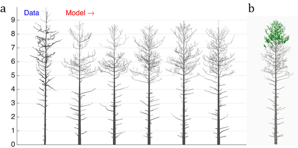
Fig. 4. The 16-parameter optimization of the stochastic LIGNUM model against a real pine tree (Data): a) tree shapes of the data tree (leftmost) and five realizations of the stochastic LIGNUM trees fitted to the data, and b) a LIGNUM tree sample with foliage. The data do not include information on foliage. The five “cloned” stochastic tree models all resemble each other in form, but differ in details. The optimal LIGNUM parameters estimated: LR = N(0.01,0.002), Q = N(0.11,0.03), T = 32, SL = 0.87 m, Smax = 72.4, Renv = N(0.83,0.23) m, βinit = 34.6 degree, ∆β = 5.5 degree, ∆ζ = 8.9 degree, βmax = 77.1 degree, ∆γ = 7.6 degree, Tsh = 12, µsh = 5.2, where N(x,y) denotes the normal distribution with mean x and standard deviation y. Other LIGNUM parameters are from Sievänen et al. (2008) and R = 60.0, VS = 0.02 m. See the parameter definitions in Table 1. The genetic algorithm has stopped after 24 full iterations/generations, where each generation consisted of 50 parameter sets.
First, we can see that there are certain drawbacks in the data, e.g., gaps between cylinders. Additionally, due to occlusion and distance effects the apical part of the crown is not fully captured by TLS; i.e., the crown appears to have fewer branches than in reality. Because of this, the coarseness of the model, and lack of the u plots representing the trunk information, the tree height was underestimated (error is about 7%), whereas the crown branch density and the trunk base diameter were overestimated (error for the breast height diameter estimation is about 55%). Nevertheless, the structure of the crown was decently captured, indicating that the choice of u, the parameters to estimate, and the model are sufficient for the purpose. Note also five different sample “clone” trees all simulated with the same best-fit parameters. The trees represent similar overall structure with varying details of organization emulating the intra-species diversity (Fig. 4a).
The dead branches are also present in the model, and their length profile corresponds to that of the real tree. This is due to the ad hoc stochastic shedding rules included in LIGNUM (Tsh and µsh). Although the measurements cannot provide for the foliage distribution in the tree, the model indicates that the foliage is spread at the upper part of the crown (Fig. 4b), which is plausible, given the natural conditions of this tree corresponding to the high-density tree stand.
4 Discussion
We have introduced the concept of Stochastic Structure Models (SSMs), based on the QSMs of real trees, and provided the proof-of-concept by simulations and real data. To make the SSM procedure capable of producing realistic general models of tree growth, the next steps will be to calibrate the models with a number of QSMs of trees of varying ages, include stochastic versions of fully synthetic (rather than biologically-based) flexible algorithms of structure formation such as those in Palubicki et al. (2009), experiment with various ways of introducing stochastic distributions in the synthetic or FSPM models, model various tree species, and include the effects of inter-tree competition required for the construction of the SSMs of entire forests. For example, the choices of Ds, the stochastic model parameters, and the coordinate planes u are not unique and may depend on the species (and are in any case somewhat simplified in this initial study). Also, controlled experiments should be carried out to test the hypotheses and assumptions behind Ds, u, and p. For example, one could expect that cloned trees grown in similar circumstances should have smaller mutual Ds than others, and the Ds of clones should correlate with environmental variation (e.g., provenance studies).
We have introduced our concept to initiate an extensive program that requires a considerable amount of experimenting by a sizable collaboration network. For this purpose, our source code is downloadable from SSMLignumSF (2015). We emphasize that the technical choices in the code and the examples here are just one sample of a large number of options. To speed up the computations, parallel computing is highly recommended: this is easy to carry out, e.g., for the members of the trial populations used in the genetic algorithm. The optimization can take tens of hours of CPU time, so a cluster or cloud implementation reduces the real-time computational cost considerably.
The program code used in this work is available at: http://github.com/inuritdino/SFennica-Lignum-SSM.
Acknowledgments
We are thankful to Sanna Kaasalainen for providing us with the TLS data and Risto Sievänen, Jari Perttunen, and Wojtek Palubicki for the valuable discussion on implementing the stochastic version of LIGNUM.
References
Åkerblom M., Raumonen P., Kaasalainen M., Casella E. (2015). Analysis of geometric primitives in quantitative structure models of tree stems. Remote Sensing 7: 4581–4603. http://dx.doi.org/10.3390/rs70404581.
Bornhofen S., Lattaud C. (2009). Competition and evolution in virtual plant communities: a new modeling approach. Natural Computing 8(2): 349–385. http://dx.doi.org/10.1007/s11047-008-9089-5.
De Reffye P., Edelin C., Françon J., Jaeger M., Puech C. (1988). Plant models faithful to botanical structure and development. Computer Graphics 22(4): 151–158. http://dx.doi.org/10.1145/378456.378505.
Fisher J. (1992). How predictive are computer simulations of tree architecture? International Journal of Plant Science 153: 137–146. http://dx.doi.org/10.1086/297071.
Honda H. (1971). Description of the form of trees by the parameters of the tree-like body: effects of the branching angle and the branch length on the shape of the tree-like body. Journal of Theoretical Biology 31: 331–338. http://dx.doi.org/10.1016/0022-5193(71)90191-3.
Kaasalainen M. (2008). Dynamical tomography of gravitationally bound systems. Inverse Problems and Imaging 2: 527–546. http://dx.doi.org/10.3934/ipi.2008.2.527.
Lu M., Nygren P., Perttunen J., Pallardy S., Larsen D. (2011). Application of the functional-structural tree model LIGNUM to growth simulation of short-rotation eastern cottonwood. Silva Fennica 45(3): 431–474. http://dx.doi.org/10.14214/sf.450.
Mäkelä A., Hari P. (1986). Stand growth model based on carbon uptake and allocation in individual tress. Ecological Modelling 33: 315–331. http://dx.doi.org/10.1016/0304-3800(86)90041-4.
Palubicki W., Horel K., Longay S., Runions A., Lane B., Mech R., Prusinkiewicz P. (2009). Self-organizing tree models for image synthesis. ACM Transactions on Graphics 28(3), Article No. 58. http://dx.doi.org/10.1145/1531326.1531364.
Perttunen J., Sievänen R., Nikinmaa E., Salminen H., Saarenmaa H., Väkevä J. (1996). LIGNUM: a tree model based on simple structural units. Annals of Botany 77: 87–98. http://dx.doi.org/10.1006/anbo.1996.0011.
Perttunen J., Sievänen R., Nikinmaa E. (1998). LIGNUM: a model combining the structure and the functioning of trees. Ecological Modelling 108: 189–198. http://dx.doi.org/10.1016/S0304-3800(98)00028-3.
Perttunen J., Nikinmaa E., Lechowicz M., Sievänen R., Messier C. (2001). Application of the functional-structural tree model LIGNUM to sugar maple saplings (Acer saccharum Marsh) growing in forest gaps. Annals of Botany 88: 471–481. http://dx.doi.org/10.1006/anbo.2001.1489.
Pfeifer N., Gorte B., Winterhalder D. (2004). Automatic reconstruction of single trees from terrestrial laser scanner data. The International Archives of the Photogrammetry, Remote Sensing and Spatial Information Sciences 35(B5): 114–119.
Prusinkiewicz P., Lindenmayer A. (1990). The algorithmic beauty of plants. Springer-Verlag, New York. http://dx.doi.org/10.1007/978-1-4613-8476-2.
Prusinkiewicz P., Mündermann L., Karwowski R., Lane B. (2001). The use of positional information in the modeling of plants. Proceedings of SIGGRAPH 2001. p. 289–300. http://dx.doi.org/10.1145/383259.383291.
Raumonen P., Kaasalainen M., Åkerblom M., Kaasalainen S., Kaartinen H., Vastaranta M., Holopainen M., Disney M., Lewis P. (2013). Fast automatic precision tree models from terrestrial laser scanner data. Remote Sensing 5: 491–520. http://dx.doi.org/ 10.3390/rs5020491.
Raumonen P., Casella E., Calders K., Murphy S., Åkerblom M., Kaasalainen M. (2015). Massive-scale tree modelling from TLS data. ISPRS Annals of the Photogrammetry, Remote Sensing and Spatial Information Sciences, II-3W4, 189–196. http://dx.doi.org/10.5194/isprsannals-II-3-W4-189-2015.
Rutzinger M., Pratihast A., Oude Elbernik S. (2011). Tree modelling from mobile laser scanning data-sets. The Photogrammetric Record 26(135): 361–372. http://dx.doi.org/10.1111/j.1477-9730.2011.00635.x.
Sievänen R., Perttunen J., Nikinmaa E., Kaitaniemi P. (2008). Toward extension of a single tree functional-structural model of Scots pine to stand level: effect of the canopy of randomly distributed, identical trees on development of tree structure. Functional Plant Biology 35: 964–975. http://dx.doi.org/10.1071/FP08077.
SSMLignumSF (2015). http://github.com/inuritdino/SFennica-Lignum-SSM. [Cited 17 Sept 2015].
Ulam S. (1962). On some mathematical properties connected with patterns of growth of figures. Proceedings of Symposia on Applied Mathematics 14: 215–224. http://dx.doi.org/10.1090/psapm/014/9947.
Weber J., Penn J. (1995). Creation and rendering of realistic trees. Proceedings of SIGGRAPH 1995: 119–128. http://dx.doi.org/10.1145/218380.218427.
Total of 22 references.
