Lingbo Dong,
Pete Bettinger,
Huiyan Qin,
Zhaogang Liu 
Reflections on the number of independent solutions for forest spatial harvest scheduling problems: a case of simulated annealing
Dong L., Bettinger P., Qin H., Liu Z. (2018). Reflections on the number of independent solutions for forest spatial harvest scheduling problems: a case of simulated annealing. Silva Fennica vol. 52 no. 1 article id 7803. https://doi.org/10.14214/sf.7803
Highlights
- No one particular neighborhood search technique of simulated annealing was found to be universally acceptable
- The optimal number of independent solutions necessary for addressing the area restriction harvest scheduling model was described with a negative logarithmic function that was related with the problem size. However, optimal number of independent solutions necessary was not sensitive to the problem size for non-spatial and unit restriction harvest scheduling model problems, which should be somewhat above 250 independent runs
- The types of adjacency constraints have moderate effects on the number of independent solutions, but these effects are not significant.
Abstract
To assess the quality of results obtained from heuristics through statistical procedures, a number of independently generated solutions to the same problem are required, however the knowledge of how many solutions are necessary for this purpose using a specific heuristic is still not clear. Therefore, the overall aims of this paper are to quantitatively evaluate the effects of the number of independent solutions generated on the forest planning objectives and on the performance of different neighborhood search techniques of simulated annealing (SA) in three increasing difficult forest spatial harvest scheduling problems, namely non-spatial model, area restriction model (ARM) and unit restriction model (URM). The tested neighborhood search techniques included the standard version of SA using the conventional 1-opt moves, SA using the combined strategy that oscillates between the conventional 1-opt moves and the exchange version of 2-opt moves, and SA using the change version of 2-opt moves. The obtained results indicated that the number of independent solutions generated had clear effects on the conclusions of the performances of different neighborhood search techniques of SA, which indicated that no one particular neighborhood search technique of SA was universally acceptable. The optimal number of independent solutions generated for all alternative neighborhood search techniques of SA for ARM problems could be estimated using a negative logarithmic function based on the problem size, however the relationships were not sensitive (i.e., 0.13 < p < 0.78) to the problem size for non-spatial and URM harvest scheduling problems, which should be somewhat above 250 independent runs. The types of adjacency constraints did moderately affect the number of independent solutions necessary, but not significantly. Therefore, determining an optimal number of independent solutions generated is a necessary process prior to employing heuristics in forest management planning practices.
Keywords
simulated annealing;
forest management planning;
combinatorial optimization;
neighborhood search;
adjacency constraint
- Dong, College of Forestry, Northeast Forestry University, Harbin 150040, China E-mail farrell0503@126.com
- Bettinger, Warnell School of Forestry and Natural Resources, University of Georgia, Athens 30602, GA, USA E-mail pbettinger@warnell.uga.edu
- Qin, College of Economic and Management, Northeast Forestry University, Harbin 150040, China E-mail huiyanqin@hotmail.com
-
Liu,
College of Forestry, Northeast Forestry University, Harbin 150040, China
E-mail
lzg19700602@163.com
Received 9 September 2017 Accepted 15 January 2018 Published 17 January 2018
Views 134505
Available at https://doi.org/10.14214/sf.7803 | Download PDF

1 Introduction
The need to protect wildlife habitat, improve water quality, preserve biodiversity, and produce wood products has resulted in a complex forest management planning environment, especially when considering the interactions among the threefold values (i.e., economic, ecological and social) of forest ecosystems. The spatial structure of the forested landscape, as well as the attributes described at the stand-level, might have an influence on ecological processes and the numerous plant and animal species living in forests (Borges and Hoganson 2000; Kurttila 2001; Wu 2004; Zeng et al. 2010). Therefore, there has been an increasing effort to develop tools by which spatial objectives can be explicitly integrated into forest planning processes. Depending on the methods used to merge spatial objectives into the forest planning process, the abundant published articles can be classified into two categories: exogenous and the endogenous optimization (Kurttila 2001). Usually, exogenous methods do not include any spatial information in their optimization process, but take into account predetermined spatial constraints (Naesset 1997; MacLean et al. 2001; Zeng et al. 2007), such as riparian zones and key habitats. However, endogenous optimization processes can employ some decision variables which describe the spatial structure of forest landscape, thus the layout of forest plans can address the constraints for the problem formulated (Borges and Hoganson 2000; McDill et al. 2002; Öhman and Lämås 2003; Crowe and Nelson 2005; Borges et al. 2015a). Since endogenous methods can generate plans that are more appropriate for long-term forest planning and thus more effective from economic and ecological points of view, there is a considerable interest in using these to solve forest planning problems in this context.
In forest planning practices, three important strategic options usually employed in forest harvest scheduling problems might be the imposition of ending inventory constraints, harvest flow constraints, and adjacency constraints (McDill et al. 2002; Zhu and Bettinger 2008). Ending inventory constraints can prevent the over-harvesting from a forest during the time horizon of a forest plan, thus may be helpful in achieving sustainable development goals of forest ecosystems. Harvest flow constraints help to produce a reasonable yield pattern over time (Bettinger et al. 2007; Borges et al. 2015a), and are often recognized as important to ensure full utilization of equipment and labor (Martins et al. 2014). A variety of spatial constraints that involve adjacency issues have been integrated into forest plans, such as those restricting the size of final harvest areas (Bettinger et al. 2003; Borges et al. 2015a), encouraging the formation of overmature forest (Kurttila et al. 2002; Kašpar et al. 2015), and promoting the clustering of harvest activities (Öhman and Lämås 2003; Smaltschinski et al. 2012). Constraining the size of final harvest openings has been the focus of much research, in which the unit restriction model (URM) and area restriction model (ARM) are the most commonly used approaches (Murray 1999). When using the URM, arbitrary adjacency units cannot be assigned a final harvest treatment in the same (or near) periods. However, when using the ARM, adjacent units may be allowed to be simultaneously harvested as long as their combined area does not exceed the maximum open area (MOA). A near time period is developed from the green-up window, which typically reflects the number of years required for adjacent final harvests to “green-up” due to reforestation practices. These are called the green-up constraints, and can be treated as a time buffer, i.e., a minimum passage of time before adjacent units can be harvested. In practice, if the mean size of management unit (MU) within a forest landscape is similar (or near) to the MOA, then the URM should be employed preferentially, while the ARM may be more suitable for the planning problems where the size of each MU is well below the MOA (Borges et al. 2015a, 2015b). Due to the combinatorial nature of these approaches, the ARM is usually more difficult to formulate and solve than the URM, but can result in a higher net present value due to the flexibility it provides in scheduling activities across a landscape (Boston and Bettinger 2006; Dong et al. 2015). Obviously, planning problems that include these constraints have non-linearity, non-continuity and non-convexity characteristics, which contribute to the problems becoming too complicated to solve effectively with exact optimization approaches. Recent works in this area using mathematical programming have provided some enhanced approaches to mitigate this issue, such as path formulation (McDill et al. 2002; Tóth et al. 2013), bucket formulation (Constantino et al. 2008; Goycoolea et al. 2009; Tóth et al. 2013), cluster packing formulation (Tóth et al. 2013) and generalized management units formulation (McDill et al. 2002; Tóth et al. 2013). However, problems may still be difficult to formulate and solvers can require considerable time to process, as these issues highly depend on the size and the complexity of planning problems.
In forestry, Kurttila (2001), Bettinger and Chung (2004), Baskent and Keles (2005), Shan et al. (2009) and Jin et al. (2016) have systematically reviewed the developmental trends in spatial forest planning problems during the last few decades, and found that heuristics, as an alternative forest plan development strategy, have drawn much as much attention as traditional mathematical programming approaches (e.g., linear programming (LP) and mixed integer programming (MIP)) for addressing complex forest planning problems. However, heuristics only can provide satisfactory, near-optimal solutions to problems rather than guaranteeing the optimal solution, mainly due to the search behavior inherent in each. Therefore, evaluating and validating the quality of solutions generated by heuristics is one of the most important processes when employing these in the development of management plans (Bettinger et al. 2003; Pukkala et al. 2003) or when comparing the performance of different heuristics (Bettinger et al. 2002; Falcão and Borges 2002; Pukkala and Kurttila 2005; Dong et al. 2015). As Bettinger et al. (2009) summarized, there are five different ways to evaluate the quality of heuristics: 1) using statistics associated with independent runs as a self-validation process; 2) comparing solution values with those generated by other heuristics; 3) comparing solution values with an estimated global optimum solution; 4) comparing solution values with relaxed LP (or MIP) solutions; 5) comparing solution values with exact LP (or MIP) solutions. Therefore, understanding the number of independent runs (or solutions) necessary is an important prerequisite for employing heuristics. However, to our best knowledge, few previous studies have focused on the question of how many independent solutions are necessary and appropriate to assess the performance of a heuristic. Based on an extensive literature review of the applications of heuristics in forest planning research, we have successfully located 68 peer-reviewed papers which have clearly declared the specific number of independent solutions generated in their papers. The statistical results showed that the number of independent solutions generated ranged from 3 to 500, with a mean value of 47.25 and a standard deviation of 68.87. Given the broad range of this assumption (independent solutions generated), it therefore seems meaningful to determine whether an optimal value exists for forest planning problems.
Simulated annealing (SA) belongs to a group of local search, s-metaheuristic processes. SA was initially introduced by Kirkpatrick et al. (1983) as a technique for solving optimization problems in fields such as electronics, transportations, medicine, etc., however, it was inspired by the work of Metropolis et al. (1953). In forest planning, SA has been used to provide a set of detailed information about where, when and how forest management prescriptions should occur (Lockwood and Moore 1993; Bachmatiuk et al. 2015), to evaluate the transportation of various forest products (Richards and Gunn 2000; Contreras et al. 2008), and to maximize the overall benefits of various conflicting management objectives (Bettinger et al. 2003; Baskent and Keles 2009). However, SA has usually been implemented using a 1-opt search process in most cases in forestry, where a new candidate solution is generated by altering the status (i.e., harvest time or prescription) of just one MU. In recent research designed to improve the performance of heuristics using alternative neighborhood search strategies, two efficient methodologies are proposed: 2-opt moves that randomly (a) change or (b) exchange the status of two different MUs. Using tabu search as an example, the exchange version of 2-opt moves in combination with a conventional 1-opt move search strategy was initially described in Bettinger et al. (1999) for forest spatial harvest scheduling problems, and then was evaluated for wildlife habitat development (Bettinger et al. 2002) and forest landscape planning problems (Bettinger et al. 2007). As compared to 1-opt moves alone, a heuristic process using this will observe smaller changes to the objective function value, thus increasing the probability that it can produce high quality forest plans not located by a conventional 1-opt move heuristic process. However, to our best knowledge, few examples of literature have implemented it with a SA algorithm. The change version of 2-opt moves, as an alternative enhancement technique, has also been used in a widespread manner during the last decade. For instance, Caro et al. (2003), Heinonen and Pukkala (2004) and Dong et al. (2015) all employed this strategy in forest spatial harvest scheduling problems with a set of metaheuristic techniques, including Monte Carlo integer programming, the Hero algorithm, tabu search, and SA. Typically, this strategy may result in a relatively larger change to objective function values than conventional 1-opt moves alone. As compared to the exchange version of 2-opt moves, the changes version does not require separate sets of 1-opt moves to increase the diversity of the solution being developed. The performance of these alternative search processes of SA in a forest spatial harvest-scheduling problem have recently been evaluated by Dong et al. (2015); the results indicated that the exchange version of 2-opt moves may be superior to the change version. However, the effects of constraint types and the problem size on their conclusions were not considered.
The goals of this paper are therefore to quantitatively evaluate the effects of the number of independent solutions generated on the performance of different neighborhood search processes of SA when solving forest harvest scheduling problems. The planning problems were formulated to maximize scheduled harvest volume over a 50 year time horizon, using ten 5-year time periods. The problem is subject to non-spatial constraints (wood flow and ending inventory), as well as URM and ARM adjacency constraints. Using SA as the base heuristic approach, the search processes included three different neighborhood search techniques, namely the standard version of SA using the conventional 1-opt moves (Method 1), SA using a combined strategy of conventional 1-opt moves and the exchange version of 2-opt moves (Method 2), and SA using the change version of 2-opt moves (Method 3). Each were applied to five different sizes of hypothetical forests. Our hypotheses were as follows: 1) the number of independent solutions generated has an effect on conclusions of the performance of a heuristic; 2) the optimal number of independent solutions necessary is related to the problem size; and 3) the type of adjacency constraints employed have an effect on the optimal number of independent solutions necessary.
2 Materials and methods
2.1 General model
To evaluate the effects of problem size on the optimal number of independent solutions generated of SA, five hypothetical forest datasets were created to represent five alternative planning problems. The problems were arranged in square grids of 20, 40, 60, 80 and 100 rows and columns, respectively. Each cell in each grid represented a 10 ha logging unit. The age for each unit was created using a random number generator, and the age varied uniformly between 0and 50 years. The management decisions we considered only included clear-cut harvests and no harvest. All of the harvest activities were assigned to the middle of a planning period. Forests can not be harvested before it reached 30 years old according to the Technical Regulations of Forest Resources Continuous Investigation in China (State Forestry Bureau 2014). Forest timber yields were estimated using the Richards equations for Dahurian larch (Larix gmelini) plantations in northeast China (Rong et al. 2011):
![]()
, where V is the predicted volume, t is the age of management unit; a = 244.22, b = 0.09 and c = 12.13 are estimated parameters of the Richards equations.
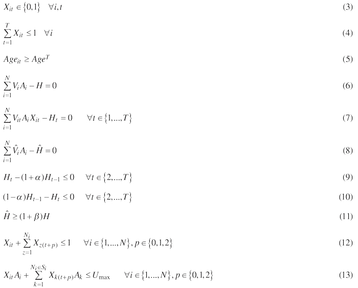
The forest planning problems that we investigated involved maximization of timber volume scheduled for harvest from a forest landscape over a 50 year planning horizon that was divided into ten 5-year time periods. These problems mainly included the ending inventory constraints, the harvest flow constraints, and the adjacency constraints. Therefore, the mathematical formulations of the tested problems were expressed as:

subject to
, where
T is the number of periods in the planning horizon
N is the number of management units in the forest
i is an arbitrary management unit
t is an arbitrary time period
m is a near-time period of the period t
z is a management unit that is adjacent to unit i
k is a management unit from a subset of units adjacent to unit i and the neighbors of unit i and so on (Murray 1999), in the form of a recursive function
Ai is the area of management unit i in hectares
Xit is a binary variable (0 or 1) indicating whether unit i is scheduled for harvest during time period t
Vi is the volume per hectare of the beginning inventory in unit i
![]() is the volume per hectare of the ending inventory in unit i
is the volume per hectare of the ending inventory in unit i
Vit is the scheduled harvest volume per hectare in unit i during time period t
H is the total volume of the beginning inventory
Ht is the total wood volume scheduled for harvest in period t
![]() is the total volume of the ending inventory
is the total volume of the ending inventory
α is the deviation proportion allowed in harvest volume from one period to the next, which was assumed as 15% in this analysis
β is the increased proportion of the total volume of the ending inventory to the beginning inventory, which was assumed as 20% in our analysis
p is the length of green-up constraints among adjacency harvest units in years
Ni is the set of all harvest units adjacent to unit i
Si is the set of all harvest units adjacent to units (Ni) that are adjacent to unit i
Umax is the maximum opening size assumed, which was assumed as 50 ha (i.e., five logging units) in this analysis
Ageit is the age of management units i in the period t
AgeT is the minimum harvest age, which was assumed as 30 years in this analysis
Eq. 2 defines the objective of maximizing timber harvested within the entire time horizon. Eq. 3 states the binary requirements on decision variables. Eq. 4 represents the singularity constraints, which prevent a unit from being harvested more than once during the entire planning horizon. Eq. 5 ensures that the minimum harvest age will not be violated. Eqs. 6–8 represent the accounting rows to add up the volume of beginning inventory (H), and scheduled for harvest for each period (Ht), and ending inventory (![]() ), respectively. Inequalities 9 and 10 define the wood flow constraints for scheduled harvests over the planning horizon, which may ensure the sustainability of the forest. Eq. 11 ensures that the ending inventory target is met. Eq. 12 represents a unit restriction model of harvest adjacency, which prohibits the neighboring units from being scheduled for a final harvest during the same time period (Murray 1999). Eq. 13 defines an area restriction model of harvest adjacency, which ensures that the size of harvested contiguous units does not exceed the maximum clear-cut opening size (Murray 1999). The adjacency constraints also hold for a 2-period green-up constraint, which can guarantee a time buffer between the locations of two final harvest units.
), respectively. Inequalities 9 and 10 define the wood flow constraints for scheduled harvests over the planning horizon, which may ensure the sustainability of the forest. Eq. 11 ensures that the ending inventory target is met. Eq. 12 represents a unit restriction model of harvest adjacency, which prohibits the neighboring units from being scheduled for a final harvest during the same time period (Murray 1999). Eq. 13 defines an area restriction model of harvest adjacency, which ensures that the size of harvested contiguous units does not exceed the maximum clear-cut opening size (Murray 1999). The adjacency constraints also hold for a 2-period green-up constraint, which can guarantee a time buffer between the locations of two final harvest units.
For testing purposes, we developed three different planning problems to assess the impacts of the number of independent solutions generated on the performances of different heuristics. These problems were constructed by adding constraints one at the time. The first planning problem referred to the non-spatial goals, which included, among others, the wood flow and ending inventory constraints (Eqs. 2–11). In the second planning problem, the URM restriction (Eq. 12) was further added, and for the third problem Eq. 12 was replaced by the ARM restriction (Eq. 13). As described here, the constraints involved in these planning problems might also be associated with forest management practices, regulations, and verification programs throughout the world. The three planning problems are named the non-spatial, URM and ARM problems consistently throughout our analysis.
2.2 Simulated annealing
Three different neighborhood search processes of SA were employed to solve the forest harvest scheduling problems. The first search process (Method 1) utilizes conventional 1-opt moves. To generate a feasible candidate solution, each 1-opt move consists of three steps: 1) changing the harvest prescription or time for just one MU; 2) verifying the practicability of the new candidate solution with respect to all constraints; 3) assessing the acceptability of the objective function value of the new candidate solution with respect to the Boltzman formula (i.e., e(–ΔE/t)). The necessary parameters for implementing SA are the starting temperature (st), the final temperature (ft), the cooling rate (cr) and the number of iterations allowed at each temperature (nrep). To illustrate the context of these parameters, a concise outline of the conventional of SA were presented in Table 1.
| Table 1. The general description of simulated annealing (SA) algorithm. |
| 1: Set SA parameters: start temperature (st), the final temperature (ft), the cooling rate (cr) and the number of iterations allowed at each temperature (nrep), and select the search strategy to generate candidate solution. 2: Generate an initial feasible solution by assigning a random prescription to each management unit (MU). Set this solution as the current (S) and best solution (S*). 3: Compute the objective function value of S. 4: Generate a candidate solution (S’) based on the current solution S by randomly selecting n MUs according to the search strategies, and then randomly change (i.e., Method 1 and Method 3) or just exchange their prescriptions (i.e., Method 2) of different MUs. 5: Check the conformity of the new candidate solution (S’) to constraints 4 and 5 in the planning formulation (see Section 2.1 for details). If feasible, go to step 6; otherwise, return to step 4. 6: Evaluate the feasibility of candidate solution S’ against the harvest even-flow (i.e., Eqs. 9–10), ending inventory (i.e., Eq. 11) and adjacency constraints (i.e., Eqs. 12–13; see Section 2.1 for details). If infeasible, reject the candidate solution, and go back to step 4. 7: Compute the objective function value of S’. 8: If the objective function value of S’ is larger than that of S*, go to step 9. Otherwise, go to step 10. 9: Let S = S’ and S* = S’, and move to step 10. 10: Evaluate the acceptability of the candidate solution S’ with respect to the objective function value, i.e., compare the result between the value of Boltzman formula (i.e., e(–∆E/t)) and a random number that varies between 0 and 1, in which ∆E is the difference between S’ and S*, and t is the current temperature. 11: If the non-improving solution is rejected, then directly go to step 12. Otherwise, let S = S’, and go to step 12. 12: If nrep is not reached, increase nrep by one, and go back to step 4. Otherwise, cool the temperature according to cooling rate cr and reset nrep to zero, and go to step 13. 13: If ft is not reached, then go back to step 4. Otherwise, output the best solution S*. |
The second search process (Method 2) will oscillate the search process back and forth between conventional 1-opt moves and the exchange version of 2-opt moves, which was initially presented by Bettinger et al. (1999). As emphasized here, the conventional 1-opt moves and the exchange version of 2-opt moves must be employed together in an independent run. A set of the conventional 1-opt moves must be firstly employed to diversity the search, and then a set of the exchange version of 2-opt moves are implemented to intensify the search. A candidate solution of the exchange version of 2-opt moves will be generated by exchanging the harvest prescription or time for two MUs simultaneously. Then, the practicability and acceptability of the candidate solution will be further evaluated according the procedure as implemented in Method 1. For the third search process (Method 3), we utilize the change version of 2-opt moves provided by Caro et al. (2003), Heinonen and Pukkala (2004) and Dong et al. (2015). The new candidate solution in this strategy will be generated by randomly changing the harvest prescription or time for two MUs simultaneously, in which the 1-opt moves can be absent.
For each search strategy, the potential change for each move will be rejected prior to assessing the impacts on the objective function value if the potential change in treatment schedules violates any one of the constraints, essentially generating an infeasible solution. This strategy avoids the need to penalize the objective function for infeasibilities, and maintains the search within the bounds of the feasible solution space.
To minimize the effects of parameter values on the performance of SA, a formal treatment for the selection of the initial parameters of SA should be included. In forestry, some research has suggested the initial parameters of SA may be related to the planning problems, such as the initial temperature and annealing rate (Heinonen and Pukkala 2004; Strimbu and Paun 2013) or the algorithm termination assumption (or freezing temperature) (Baskent and Jordan 2002). However, these aspects of a heuristic search may be difficult to employ directly in our research, due to the different planning formulations. In addition, it may be too time-consuming to implement a new parameter sensitivity analysis in this paper. Therefore, a wide range of the combinations among the four important parameters of SA were evaluated using trial-and-error tests, as implemented in Bettinger et al. (2002). The four SA parameters we used for this problem were: st = 106, ft = 10, cr = 0.99 and nrep = 100, which resulted in 114 600 iterations per independent run. The solutions of the planning problems were generated using software developed within Microsoft Visual Basic 6.0, and applied on a 2.6 GHz Core i5 processor computer that used the Windows 7 Pro 32 Bits operating system.
2.3 Analytical method
The main objective of this study was to analyze whether the number of independent runs of a heuristic has a significant effect on conclusions regarding the performance of the heuristic. We delve into this using three s-metaheuristic neighborhood search strategies involving SA, as applied to three increasing difficult harvest scheduling problems. One thousand feasible solutions for each of 45 planning problem instances (i.e., 3 harvest scheduling problems × 3 SA search strategies × 5 forest datasets) were generated, where which each was initiated from a random, feasible starting solution. Therefore, a total of 45 000 independent solutions were generated for this analysis, which required a total computation time of approximately 1500 h (about 62 days). All of the solutions were sorted strictly along the chronological order of the solutions generated. The 1000 independent solutions of each problem instance were grouped into 20 sets along the chronological order of the solutions generated. The first set consisted of the first 50 runs (of the 1000 independent solutions of a problem instance) and the other sets were formed by successively adding 50 more runs, that is, the first set consisted of runs 1–50, the second set consisted of runs 1–100, the third set consisted of runs 1–150, and so on. The time of discovery of the superior solution (which might be treated as the near-optimal solution) for a specific planning problem instance is usually a random event within a single search process, and depends on the parameters employed, their status (if they change), search strategies inherent in the heuristic, and the complexities of the planning problem. Therefore, it may be more practical to evaluate the search capabilities of heuristics using average objective function values of the best solutions located during a heuristic search process (i.e., the final solution for each independent run) rather than the potential maximum values. The another reason for using the average values instead of maximum values to evaluate the performance of different implementation of SA is that the average values of a set of mean solutions is more stable than the maximum values (which are usually), which highly depend on the search mechanism of alternative neighborhood search techniques of SA. Therefore, the developments of the mean objective function values for each group of three alternative neighborhood search strategies related to the group number were presented on scatter plot in this context, which are employed to verify our first hypothesis. Then, we can conclude that the number of independent solutions may have effects on the stated performance of different neighborhood search techniques if any two curves have one or more intersection points on the scatter plot.
3 Results
The maximum, minimum, means and standard deviations of objective function values of the independent solutions all indicated that no one particular neighborhood search technique was universally acceptable, given the number of decision variables and the constraint types assumed in the planning formulations (Table 2). With respect to objective function values, Method 3 found the largest minimum solutions (best solutions) for 12 out of 15 cases (80%), however the other three cases were all generated by Method 2. For maximum solutions, the largest maximum solutions were found on 12 out of 15 cases (80%) by Method 3, and 2 out of 15 cases (13%) by Method 2, and only 1 case by Method 1. For mean solutions, the largest mean solution values were found on 7 out of 15 cases (approximately 47%) by Method 1, and 2 out of 15 cases (approximately 13%) by Method 2, however the other six cases were all located by Method 3. For standard deviations, the smallest standard deviations values were found on 7 out of 15 cases (47%) by Method 2, and 6 out of 15 cases (40%) by Method 3, and only 2 cases were observed by Method 1.
| Table 2. The statistical results of 1000 independent objective function values (106 m3) of the three planning problems for each hypothetical forest dataset when using three different neighborhood search techniques of simulated annealing (SA). The largest minimum objective function value for each planning scenario is highlighted in italic, the maximum objective function value is highlighted in boldface, the maximum mean objective function value is highlighted with a shadow, and the smallest standard deviation (SD) value is highlighted with underline. Method 1 represents the standard version of SA using 1-opt moves, Method 2 represents the exchange version of SA using 2-opt moves, and Method 3 represents the change version of SA using 2-opt moves. NON represents the non-spatial planning problems, URM represents the unit restriction model, ARM represents the area restriction model. | ||||||||||||||
| Forest | Model | Method 1 | Method 2 | Method 3 | ||||||||||
| Min. | Max. | Mean | SD | Min. | Max. | Mean | SD | Min. | Max. | Mean | SD | |||
| 400 | NON | 0.558 | 0.623 | 0.572 | 0.013 | 0.561 | 0.634 | 0.574 | 0.013 | 0.560 | 0.638 | 0.575 | 0.014 | |
| ARM | 0.553 | 0.622 | 0.567 | 0.013 | 0.555 | 0.630 | 0.568 | 0.012 | 0.556 | 0.637 | 0.568 | 0.013 | ||
| URM | 0.457 | 0.598 | 0.486 | 0.023 | 0.460 | 0.598 | 0.488 | 0.023 | 0.463 | 0.612 | 0.489 | 0.024 | ||
| 1600 | NON | 2.217 | 2.602 | 2.267 | 0.083 | 2.222 | 2.616 | 2.266 | 0.074 | 2.224 | 2.635 | 2.267 | 0.072 | |
| ARM | 2.127 | 2.577 | 2.201 | 0.080 | 2.136 | 2.587 | 2.197 | 0.064 | 2.137 | 2.607 | 2.202 | 0.066 | ||
| URM | 1.714 | 2.420 | 1.847 | 0.084 | 1.706 | 2.441 | 1.848 | 0.081 | 1.720 | 2.448 | 1.855 | 0.083 | ||
| 3600 | NON | 4.887 | 5.744 | 5.041 | 0.260 | 4.894 | 5.752 | 5.005 | 0.208 | 4.892 | 5.800 | 4.980 | 0.168 | |
| ARM | 4.741 | 5.683 | 4.910 | 0.218 | 4.757 | 5.673 | 4.872 | 0.139 | 4.766 | 5.727 | 4.897 | 0.180 | ||
| URM | 3.859 | 4.692 | 4.288 | 0.174 | 3.814 | 4.687 | 4.280 | 0.182 | 3.866 | 5.338 | 4.285 | 0.181 | ||
| 6400 | NON | 8.790 | 10.237 | 9.102 | 0.508 | 8.794 | 10.482 | 9.042 | 0.488 | 8.809 | 10.499 | 9.025 | 0.457 | |
| ARM | 8.258 | 10.086 | 8.778 | 0.579 | 8.306 | 10.303 | 8.603 | 0.440 | 8.331 | 10.304 | 8.617 | 0.437 | ||
| URM | 6.860 | 8.183 | 7.631 | 0.298 | 6.862 | 8.172 | 7.660 | 0.299 | 6.897 | 8.154 | 7.647 | 0.283 | ||
| 10000 | NON | 13.675 | 15.620 | 14.319 | 0.795 | 13.695 | 16.212 | 14.141 | 0.832 | 13.719 | 16.274 | 14.178 | 0.863 | |
| ARM | 12.782 | 15.475 | 13.946 | 1.010 | 12.913 | 15.983 | 13.490 | 0.856 | 12.893 | 15.885 | 13.555 | 0.870 | ||
| URM | 10.705 | 12.711 | 12.007 | 0.439 | 10.873 | 12.724 | 12.028 | 0.433 | 10.887 | 12.690 | 12.050 | 0.418 | ||
The average wood volume scheduled when using the non-spatial constraints was always superior to other cases when the spatial constraints were employed (Table 2), regardless of the evaluation criterions (i.e., minimum, maximum and mean). The wood volume scheduled of the ARM and URM problems only accounted for approximately 97.13% and 84.25% respectively of that of the non-spatial problems. The coefficients of variation (CV) of all the planning scenarios were all less than 10%, but in most cases the CV values obtained by the two enhanced search process of SA were both smaller than that from Method 1 (approximately 73% cases), indicating a smaller range of objective function values were generated.
The development of mean objective function values for each group related to the number of independent solutions (i.e., the order of group) were illustrated in Fig. 1. These graphs verified that no one particular neighborhood search technique was universally optimal. The development trend within each curve fluctuated intensively with the increases in the number of independent runs, in which the values of the differences between the minimum (zmin) and maximum (zmax) average objective values relative to the minimum average objective values (i.e., (zmax–zmin)/zmin × 100) varied from 0.15% to 2.28%. For most of the planning problems, at least one or more intersection points were observed in the scatter plots. For instance, four different intersection points were observed from the curves between Method 2 and Method 3 for the non-spatial planning problems of 10 000-units dataset. However, some exceptions also occurred, such as the non-spatial planning problems for 3600-units dataset, where the variation in scheduled timber volume using Method 1 was significant larger than that of the other methods.
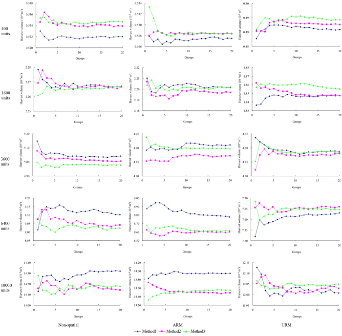
Fig. 1. The development of mean objective function value within each group of the three planning problems for the five hypothetical forest datasets when employed using three different neighborhood search techniques of simulated annealing (SA). Method 1 represents the standard version of SA using 1-opt moves, Method 2 represents the exchange version of SA using 2-opt moves, and Method 3 represents the change version of SA using 2-opt moves. Non-spatial represents the non-spatial planning problems, URM represents the unit restriction model, ARM represents the area restriction model. View larger in new window/tab.
As showed in Fig. 1, the developments of mean objective function values of each group for specific problem were always fluctuation with the increase of group order. The fluctuations of mean objective function values between two consecutive orders may be very small, or even not significant for most cases. Therefore, the maximum objective function values of the 1000 independent solutions for specific planning problem were employed to locate the optimal group orders (Fig. 2) instead of using the mean objective function values. According to Barrett et al. (1998), the group order at here can be treated as random variable, because of the appearance of the potential maximum solutions of an independent run for a specific planning problem is also a random event. In the viewpoint of this, the average values and standard deviation (SD) of the group orders for non-spatial, ARM and URM planning problems seemed to be 9.20 ± 4.46, 6.60 ± 4.72 and 7.13 ± 5.45 respectively (presented in the form of “Mean ± SD”), but the differences between them were all not significant, in which the p-values of significance testing using the paired-sample t-tests ranged from 0.13 to 0.78. For the non-spatial and URM planning problems, the optimal number of independent solutions generated for the three neighborhood search techniques of SA were all not sensitive to the problem sizes, but the optimal number of independent solutions generated of most planning instances should be somewhat above 250 runs (approximately 87% and 67% cases). However, the optimal number of independent solutions necessary all presented negative logarithmic decline trends with the increases of problem size when evaluated for the ARM problems. The relations between the optimal number of independent solutions generated (Y) and the number of forest MUs (X) can be fitted as:
ARM problem with Method 1: Y = –2.376 Ln(X) + 23.788 R2 =0.730
ARM problem with Method 2: Y = –4.145 Ln(X) + 40.573 R2 = 0.849
ARM problem with Method 3: Y = –3.644 Ln(X) + 35.808 R2 = 0.780
, where Ln() is the natural logarithmic function; R2 is the coefficient of determination between observation and fitting values.
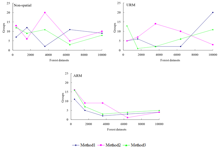
Fig. 2. The development of the group orders in which the maximum objective function values were obtained for the alternative planning problems related to the number of management units within a forest dataset, when using three different neighborhood search techniques of simulated annealing (SA). Method 1 represents the standard version of SA using 1-opt moves, Method 2 represents the exchange version of SA using 2-opt moves, and Method 3 represents the change version of SA using 2-opt moves. Non-spatial represents the non-spatial planning problems, URM represents the unit restriction model, ARM represents the area restriction model. View larger in new window/tab.
The average amount of time required to locate the maximum objective function value of each solution at the first time (not the entire search time) for the three neighborhood search techniques of SA is highly related to the problem size and constraint types (Fig. 3). The CV values of the computation time for all the planning problems varied from 40.06% to 292.90%, indicating the quality of initial solution may have significant effects on the search process of SA. For the non-spatial and ARM problems, the computation time increased significantly with the increases of problem size. However, the computation time presented a significant decline trend with the increases of problem size for URM problems. The reason for this phenomenon may be that the larger the problem size is, the more loose restricted for the planning problem, but it may be more easy to locate the satisfactory solution (not optimal solution), especially when the constraints (spatial vs. non-spatial) for one specific planning problem (i.e., Non-spatial, URM or ARM) were all consistent within different sizes of forest dataset. The amount of time required for the Method 2 was usually significant longer than that of the other methods, but the differences between Method 1 and Method 3 were difficult to distinguish.
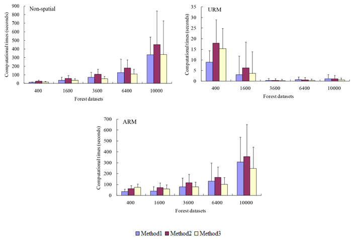
Fig. 3. The mean and standard deviation of computation time for alternative planning problems related to the number of management units within a forest dataset, when using three different neighborhood search techniques of simulated annealing (SA). Method 1 represents the standard version of SA using 1-opt moves, Method 2 represents the exchange version of SA using 2-opt moves, and Method 3 represents the change version of SA using 2-opt moves. Non-spatial represents the non-spatial planning problems, URM represents the unit restriction model, ARM represents the area restriction model. View larger in new window/tab.
4 Discussion
Our first hypothesis, that the performance of different heuristics might be vary when a different number of independent solutions was generated, appear to be supported by our results. Due to the stochastic behavior of some s-metaheuristics when generating candidate solutions, the resulting solution of heuristic method can be considered as an independent sample from a larger population. Obviously, if the sample size was inadequate, the statistical estimates (i.e., mean value and standard deviation) related to the results may be far from the true values, thus the conclusions may be not authentic. However, if the sample size becomes too large, the statistical estimates may be nearer to the true values, but it would be too costly and time-consuming to implement such an experiment. Therefore, it is necessary to determine the optimal number of independent solutions generated for specific forest planning problems. Using the different neighborhood search techniques of SA as an example, our results showed that the mean objective function values among different groups (solutions selected according to run time) only varied by 0.15% to 2.28%, but several intersection points of the most instances can be clearly observed from the curves developed for the three methods when applied to different forest planning problems (Fig. 1) which perfectly confirmed our hypothesis that no one particular neighborhood search technique was universally acceptable. However, one should keep in mind that the three neighborhood search techniques of SA all have the similar search behavior, especially for the accepting mechanism of inferior solutions. Therefore, the effects of the number of independent solutions generated on the conclusions of different heuristics algorithm, such as tabu search, threshold accepting and genetic algorithms, need further investigated in the future.
Our second hypothesis, that the number of independent solutions generated might be related to the problem size, was partly supported by our results. As one considered for a special planning problem, the larger the problem size, the more feasible combinations there would be, the larger the solution space would be, the more difficult would be to find the optimal solution, and therefore the more number of independent solutions generated may be needed to obtain reliable results. Therefore, the number of independent solutions generated may be logically related to the problem size. However, our results showed that the optimal number of independent solutions generated of the three neighborhood search techniques for non-spatial and URM problems were all not sensitive to the problem size, but the optimal optimization number presented a negative logarithmic decline trend with the increases of problem size for ARM problems (Fig. 2). In addition, previously researches also showed that the problem size may affect the solution qualities of heuristics. Crowe and Nelson (2005), for an example, reported that a weak decline trend between larger problem size and poorer mean solution qualities was observed in the area-restricted harvest scheduling problem. However, since the complexity of the constraints (the spatial aspect in particular), we did not solve the problems using the traditional MIP method to evaluate the quality of solutions in our study. Of course, some modifications have been put forward, such as path formulation, bucket formulation and generalized management unit formulation (e.g., Tóth et al. 2013), which can improve the ability of MIP methods to solve forest spatial planning problems.
The final hypothesis, that the type of adjacency constraints may also affect the optimal number of independent solutions generated, appears to be not supported by our results. The average optimal number (i.e., group order) of independent solutions for non-spatial, ARM and URM problems were 9.20 ± 4.46, 6.60 ± 4.72 and 7.13 ± 5.45 respectively, but the differences between them were all not significant (i.e., 0.13 < p < 0.78; Fig. 2). However, the type of adjacency constraints have significant effects on the economic benefits as would be expected. Results showed that the economic benefits were reduced significantly when spatial constraints were integrated into the planning models, which has already been stated by other authors (Boston and Bettinger 2001). In our case study, the harvest levels for ARM and URM problems were approximately 97.1% and 84.3% of similar non-spatial problems (Table 2). The obvious reason for this pattern is that as planning problems become more constrained, some harvesting options that violated the adjacency and green-up constraints would be prevented in nature. However, a set of stand- (e.g., site index and tree species) and forest-level variables (e.g., land size and age class distributions) may have significant effects on this pattern. For example, Borges et al. (2015b) affirmed that the formulations using a predefined variable length and the height information from the growth simulator for the green-up constraints can significantly diminish the differences between the spatial and non-spatial planning problems when compared that with the formulations using the predefined fixed length green-up time. Zhu and Bettinger (2008) found that landowners with small-sized forests that covered with young initial age class distribution would be significantly more affected by the spatial constraints. Therefore, forest managers and planners should carefully evaluate the effects of these forest- and stand-level variables on the various services and goods of forest ecosystems when employed in a specific region.
Neighborhood search techniques of s-metaheuristic have been employed for a long term, however the conclusions on the performances of them are always discrepant. For example, Caro et al. (2003), Heinonen and Pukkala (2004) and Dong et al. (2015) all have confirm that the change version of 2-opt moves were significant superior to the conventional 1-opt moves for alternative planning problems and forest datasets, however Bachmatiuk et al. (2015) recently found that changing simultaneously the prescription in more than one MU did not improve the performance of SA when the combinatorial problem became very large (213 116 decision choices) which were perfectly in line with our results for the Non-spatial and ARM planning problems when evaluated for Method 1 and Method 3 in regardless of the size of forest dataset. However, to our best knowledge, few papers have directly compared the performances of the change and exchange version of 2-opt moves, the work of Dong et al. (2016) was an exception. They reported that the performance of the exchange version of 2-opt moves was significant superior to the change version of 2-opt moves when evaluated for SA algorithm in a maximum opening size problem. Particularly, they further found that the performances of the reversion search strategy between 1-opt moves and the exchange version of 2-opt moves was the best. Different with the above mentioned strategies, Borges et al. (2014) provided some new methods of introducing biased probabilities in the MU selection, and found that they can generated higher average and maximum objective function values when compared them with the conventional method that assumed uniform probabilities (i.e., randomly). Hence, the effects of these neoteric search strategies on the optimal number of independent solutions generated and their relations with problem size still need further research.
In addition to increasing the number of independent solutions to improve the probability that heuristics will locate the optimal solution to a problem, implementing a longer run (i.e., more iteration in each independent run) for single solution may be another efficient strategy to generate a higher quality solution. Crews (2014), for an example, investigated the performances of longer single runs and many multiple shorter runs in improving the probability of SA and threshold accepting (TA) when applied to the traveling salesman problem. The results indicated that in a majority of cases, a longer single run was significantly superior to multiple shorter runs, but there were still some cases in which the multistart method outperformed single runs. However, the effects of a longer runs of single solution on forest harvest-scheduling problems and when used with other heuristic algorithms still needs further research.
5 Conclusions
With the results in our case study, we can conclude that the number of independent solutions required for solving a problem using a heuristic can have a clear effect on conclusions of the performance of the heuristic, as demonstrated when different neighborhood search techniques of SA were applied to three increasing difficult planning problems. In other words, no one particular set of assumptions concerning the SA search process could be universally accepted as the most appropriate for these harvest scheduling problems. The independent solutions generated using alternative neighborhood search techniques of SA for the ARM harvest scheduling problem were described by negative logarithmic decline trends with increases in problem size, however the trends were not sensitive to problem size for the non-spatial and the URM harvest scheduling problems. In addition, the types of adjacency constraints do moderately affect the number of independent solutions that seem necessary, but the differences between them are not significant (i.e., 0.13 < p < 0.78). Our results enlighten discussions centered on heuristic search assumptions, and suggest that comparisons of different neighborhood search techniques may be confounded if the number of independent solutions generated are not similar. For the problems under study, our hypotheses were only evaluated for the three widely used neighborhood search techniques of an s-metaheuristic, while the conclusions might be different for instances with larger number of moves or biased probabilities in the MU selection process, which we have left for further research in the future. In addition, while the mechanisms for accepting inferior solutions among the three alternative SA methods are indistinguishable, they are different from other heuristic processes, thus the conclusions may be not suitable for the comparison studies among different heuristic algorithms (e.g., tabu search, genetic algorithms).
Acknowledgments
This work was financially supported by the National Natural Science Foundation (31700562) through the College of Forestry at the Northeast Forestry University and the U.S. Department of Agriculture, National Institute of Food and Agriculture, McIntire-Stennis project (1012166), administered by the Warnell School of Forestry and Natural Resources at the University of Georgia. We also express our deepest appreciations to the anonymous reviewers for their helpful and valuable comments on this work.
References
Bachmatiuk J., Garcia-Gonzalo J., Borges J.G. (2015). Analysis of the performance of different implementations of a heuristic method to optimize forest harvest scheduling. Silva Fennica 49(4) article 1326. http://dx.doi.org/10.14214/sf.1326.
Barrett T.M., Gilless J.K., Davis L.S. (1998). Economic and fragmentation effects of clear-cut restrictions. Forest Science 44: 569–577.
Baskent E.Z., Jordan G.A. (2002). Forest landscape management modeling using simulated annealing. Forest Ecology and Management 165(1): 29–45. http://dx.doi.org/10.1016/S0378-1127(01)00654-5.
Baskent E.Z., Keles S. (2005). Spatial forest planning: a review. Ecological Modelling 188: 145–173. http://dx.doi.org/10.1016/j.ecolmodel.2005.01.059.
Baskent E.Z., Keles S. (2009). Developing alternative forest management planning strategies incorporating timber, water and carbon values: an examination of their interactions. Environmental Modeling and Assessment 14: 467–480. http://dx.doi.org/10.1007/s10666-008-9148-4.
Bettinger P., Chung W. (2004). The key literature of and trends in forest-level management planning in North America, 1950–2001. International Forestry Review 6(1): 40–50. http://dx.doi.org/10.1505/ifor.6.1.40.32061.
Bettinger P., Boston K., Sessions J. (1999). Intensifying a heuristic forest harvest scheduling search procedure with 2-opt decision choices. Canadian Journal of Forest Research 29(11): 1784–1792. http://dx.doi.org/10.1139/x99-160.
Bettinger P., Graetz D., Boston K., Sessions J., Chung W. (2002). Eight heuristic planning techniques applied to three increasingly difficult wildlife planning problems. Silva Fennica 36(2): 561–584. http://dx.doi.org/10.14214/sf.545.
Bettinger P., Johnson D.L., Johnson K.N. (2003). Spatial forest plan development with ecological and economic goals. Ecological Modelling 169: 215–236. http://dx.doi.org/10.1016/S0304-3800(03)00271-0.
Bettinger P., Boston K., Kim Y.H., Zhu J. (2007). Landscape-level optimization using tabu search and stand density-related forest management prescriptions. European Journal of Operational Research 176(2): 1265–1282. http://dx.doi.org/10.1016/j.ejor.2005.09.025.
Bettinger P., Sessions J., Boston K. (2009). A review of the status and use of validation procedures for heuristics used in forest planning. Mathematical and Computational Forestry & Natural-Resources Sciences 1(1): 26–37.
Borges J.G., Hoganson H.M. (2000). Structuring a landscape by forestland classification and harvest scheduling spatial constraints. Forest Ecology and Management 130: 269–275. http://dx.doi.org/10.1016/S0378-1127(99)00180-2.
Borges P., Eid T., Bergseng E. (2014). Applying simulated annealing using different methods for the neighborhood search in forest planning problems. European Journal of Operational Research 233(3): 700–710. http://dx.doi.org/10.1016/j.ejor.2013.08.039.
Borges P., Bergseng E., Eid T., Gobakken T. (2015a). Impact of maximum opening area constraints on profitability and biomass available in forest forestry – a large, real world case. Silva Fennica 49(5) article 1347. http://dx.doi.org/10.14214/sf.1347.
Borges P., Martins I., Bergseng E., Eid T., Gobakken T. (2015b). Effects of site productivity on forest harvest scheduling subject to green-up and maximum area restriction. Scandinavian Journal of Forest Research 31(5): 507–516. http://dx.doi.org/10.1080/02827581.2015.1089931.
Boston K., Bettinger P. (2001). The economic impact of green-up constraints in the southeastern United States. Forest Ecology and Management 145(3): 191–202. http://dx.doi.org/10.1016/S0378-1127(00)00417-5.
Boston K., Bettinger P. (2006). An economic and landscape evaluation of the green-up rules for California, Oregon and Washington (USA). Forest Policy and Economics 8(3): 251–266. http://dx.doi.org/10.1016/j.forpol.2004.06.006.
Caro F., Constantino M., Martins I., Weintraub A. (2003). A 2-opt tabu search procedure for the multiperiod forest harvesting problem with adjacency, greenup, old growth, and even flow constraints. Forest Science 49(5): 738–751.
Constantino M., Martins I., Borges J.G. (2008). A new mixed integer programming model for harvest scheduling subject to maximum area restrictions. Operations Research 56(3): 542–551. http://dx.doi.org/10.1287/opre.1070.0472.
Contreras M.A., Chung W., Jones G. (2008). Applying ant colony optimization metaheuristic to solve forest transportation planning problems with side constraints. Canadian Journal of Forest Research 38(11): 2896–2910. http://dx.doi.org/10.1139/X08-126.
Crews M. (2014). A comparison of single runs versus multistart for simulated annealing and threshold accepting. MS Thesis, Oregon State University, USA.
Crowe K.A., Nelson J.D. (2005). An evaluation of the simulated annealing algorithm for solving the area-restricted harvest-scheduling model against optimal benchmarks. Canadian Journal of Forest Research 35(10): 2500–2509. http://dx.doi.org/10.1139/x05-139.
Dong L., Bettinger P., Liu Z., Qin H. (2015). A comparison of a neighborhood search technique for forest spatial harvest scheduling problems: a case study of the simulated annealing algorithm. Forest Ecology and Management 356: 124–135. http://dx.doi.org/10.1016/j.foreco.2015.07.026.
Dong L., Bettinger P., Liu Z., Qin H., Zhao Y. (2016). Evaluating the neighborhood, hybrid and reversion search techniques of a simulated annealing algorithm in solving forest spatial harvest scheduling problems. Silva Fennica 50(4) article 1622. http://dx.doi.org/10.14214/ sf.1622.
Falcão A.O., Borges J.G. (2002). Combining random and systematic search heuristic procedures for solving spatially constrained forest management scheduling problems. Forest Science 48: 608–621.
Goycoolea M., Murray A., Vielma J.P., Weintraub A. (2009). Evaluating approaches for solving the area restriction model in harvest scheduling. Forest Science 55(2): 149–165.
Heinonen T., Pukkala T. (2004). A comparison of one- and two-compartment neighborhood in heuristic search with spatial forest management goals. Silva Fennica 38(3): 319–332. http://dx.doi.org/10.14214/sf.419.
Jin X.J., Pukkala T., Li F.R. (2016). Fine-tuning heuristic methods for combinatorial optimization in forest planning. European Journal of Forest Research 135(4): 765–779. http://dx.doi.org/ 10.1007/s10342-016-0971-x.
Kašpar J., Marušák R., Hlavatý R. (2015). A forest planning approaches with respect to the creation of overmature reserved areas in managed forests. Forests 6(2): 328–343. http://dx.doi.org/10.3390/f6020328.
Kirkpatrick S., Gelatt C.D., Vecchi M.P. (1983). Optimization by simulated annealing. Science 220(4598): 671–680. http://dx.doi.org/10.1126/science.220.4598.671.
Kurttila M. (2001). The spatial structure of forests in the optimization calculations of forest planning: a landscape ecological perspective. Forest Ecology and Management 142(1–3): 129–142. http://dx.doi.org/10.1016/S0378-1127(00)00343-1.
Kurttila M., Uuttera J., Mykrä S., Kurki S., Pukkala T. (2002). Decreasing the fragmentation of old forests in landscapes involving multiple ownership in Finland: economic, social and ecological consequences. Forest Ecology and Management 166(1–3): 69–84. http://dx.doi.org/10.1016/S0378-1127(01)00663-6.
Lockwood C., Moore T. (1993). Harvest scheduling with spatial constraints: a simulated annealing approach. Canadian Journal of Forest Research 23(3): 468–478. http://dx.doi.org/10.1139/x93-065.
MacLean D.A., Erdle T.A., MacKinnon W.E., Porter K.B., Beaton K.P., Cormier G., Morehouse S., Budd M. (2001). The spruce budworm decision support system: forest protection planning to sustain long-term wood supply. Canadian Journal of Forest Research 31: 1742–1757. http://dx.doi.org/10.1139/x01-102.
Martins I., Ye M., Constantino M., da Conceição Fonseca M., Cadima J. (2014). Modeling target volume flows in forest harvest scheduling subject to maximum area restrictions. TOP 22(1): 343–362. http://dx.doi.org/10.1007/s11750-012-0260-x.
McDill M.E., Rebain S.A., Braze J. (2002). Harvest scheduling with area-based adjacency constraints. Forest Science 48: 631–642.
Metropolis N., Rosenbluth A., Rosenbluth M., Teller A., Teller E. (1953). Equation of state calculations by fast computing machines. Journal of Chemical Physics 21: 1087–1101. http://dx.doi.org/10.2172/4390578.
Murray A.T. (1999). Spatial restrictions in harvest scheduling. Forest Science 45: 45–52.
Naesset E. (1997). A spatial decision support system for long-term forest management planning by means of linear programming and a geographical information system. Scandinavian Journal of Forest Research 12(1): 77–88. http://dx.doi.org/10.1080/02827589709355387.
Öhman K., Lämås T. (2003). Clustering of harvest activities in multi-objective long-term forest planning. Forest Ecology and Management 176(1–3): 161–171. http://dx.doi.org/10.1016/S0378-1127(02)00293-1.
Pukkala T., Kurttila M. (2005). Examining the performance of six heuristic optimization techniques in different forest planning problems. Silva Fennica 39(1): 67–80. http://dx.doi.org/10.14214/sf.396.
Pukkala T., Ketonen T., Pykäläinen J. (2003). Predicting timber harvests from private forests-a utility maximization approach. Forest Policy and Economics 5(3): 285–296. http://dx.doi.org/10.1016/S1389-9341(02)00062-X.
Richards E.W., Gunn E.A. (2000). A model and tabu search method to optimize stand harvest and road construction schedules. Forest Science 46(2): 188–203.
Rong J.T., Liu D.R., Lin Z.Z., Lei X.D. (2011). Volume growth models of main forest types in over-logged forest region, northeast China. China Forestry Science and Technology 25(1): 30–34. [In Chinese with an English abstract].
Shan Y., Bettinger P., Cieszewski C.J., Li R. (2009). Trends in spatial forest planning. Mathematical and Computational Forestry & Natural-Resources Sciences 1(2): 86–112.
Smaltschinski T., Seeling U., Becker G. (2012). Clustering forest harvest stands on spatial networks for optimised harvest scheduling. Annals of Forest Science 69(5): 651–657. http://dx.doi.org/10.1007/s13595-012-0182-7.
Strimbu B.M., Paun M. (2013). Sensitivity of forest plan value to parameters of simulated annealing. Canadian Journal of Forest Research 43(1): 28–38. http://dx.doi.org/10.1139/cjfr-2012-0277.
State Forestry Bureau (2014). Technical regulations of forest resources continuous investigation in China. State Forestry Bureau, Beijing. [In Chinese].
Sustainable Forestry Initiative (2015). SFI 2015–2019 forest management standard. Sustainable Forestry Initiative, Inc., Washington, DC.
Tóth S.F., McDill M.E., Könnyii N., George S. (2013). Testing the use of lazy constraints in solving area-based adjacency formulations of harvest scheduling models. Forest Science 59(2): 157–176. http://dx.doi.org/10.5849/forsci.11-040.
Wu J.G. (2004). The key research topics in landscape ecology. Acta Ecologica Sinica 24(9): 2074–2076. [In Chinese with an English abstract].
Zeng H., Garcia-Gonzalo J., Peltola H., Kellomäki S. (2010). The effects of forest structure on the risk of wind damage at a landscape level in a boreal forest ecosystem. Annals of Forest Science 67(1): 111–111. http://dx.doi.org/10.1051/forest/2009090.
Zeng H., Talkkari A., Peltola H., Kellomäki S. (2007). A GIS-based decision support system for risk assessment of wind damage in forest management. Environmental Modelling and Software 22(9): 1240–1249. http://dx.doi.org/10.1016/j.envsoft.2006.07.002.
Zhu J., Bettinger P. (2008). Estimating the effects of adjacency and green-up constraints on landowners of different sizes and spatial located in the southeastern U.S. Forest Policy and Economics 10(5): 295–302. http://dx.doi.org/10.1016/j.forpol.2007.11.006.
Total of 54 references.
