Luis A. Apiolaza  ,
Rosa M. Alzamora
,
Rosa M. Alzamora
Building deployment portfolios for genotypes under performance instability
Apiolaza L. A., Alzamora R. M. (2013). Building deployment portfolios for genotypes under performance instability. Silva Fennica vol. 47 no. 1 article id 901. https://doi.org/10.14214/sf.901
Abstract
We used portfolio theory to analyze the tradeoffs between returns and performance instability of deployment units for Pinus radiata D. Don. We considered three groups of 34 trees each grown to produce appearance lumber, structural lumber, or both. Risk was based on the variability of tree returns in scenarios of changing volume, wood stiffness and presence of resin defects due to genotype by environment interaction inducing both changes of scale and differential tree response to environmental scenarios. The return of structural trees was highly variable with a mean of 3.11 NZ $/stem/year, followed by appearance-structural trees (3.48 NZ $/stem/year). In contrast, appearance trees had the lowest returns (1.99 NZ $/stem/year) and variability. The portfolio model selected structural trees in high-risk scenarios, but selection was apportioned between structural and appearance-structural trees as the risk decreased. The model selected only appearance trees for high-risk aversion. The analysis also considered silvicultural regimes, where the appearance-structural regime was selected under high variability. As risk decreased the appearance grades regime was also selected. The structural regime was rarely selected due to the variability of stiffness between trees. Using genotypes improved for stiffness could increase the expected value and reduce variability for structural purposes, making the structural regime more appealing.
Keywords
Pinus radiata;
wood quality;
breeding objectives;
clonal portfolio;
deployment portfolio;
genotype by environment interaction
-
Apiolaza,
School of Forestry, University of Canterbury, Private Bag 4800, 8042 Canterbury, New Zealand
E-mail
luis.apiolaza@canterbury.ac.nz
- Alzamora, Instituto de Manejo Forestal, Universidad Austral, Valdivia, Chile E-mail ralzamor@uach.cl
Received 6 June 2012 Accepted 19 December 2012 Published 11 June 2013
Views 244971
Available at https://doi.org/10.14214/sf.901 | Download PDF

1 Introduction
Forestry firms use several approaches and time-frames to manage tree variability. For example, genetic material is bred to target specific traits that maximize value, silvicultural regimes manipulate genotypes to alter the quantity and quality of products at harvest, stands are grouped in management units for forest planning, and logs are segregated and matched to processing facilities at harvest time.
Superior genotypes are established using different deployment units that – depending on species, cost and past-experience – may include bulk material, open-pollinated families, controlled-pollinated families and clones. The performance of these units depends on their genotype, the environment where they are growing (including site and silviculture) and on the interaction between genotype and environment (GxE). In addition to current environmental conditions, firms also have to deal with projected changes in their forest estate due to climate change (e.g. Ministry for the Environment 2008; Crowe and Parker 2008). Firms should then account for both predicted genetic superiority and the risk introduced by performance instability when deploying genotypes.
‘Clonal portfolios’ – loosely defined as a portfolio of deployment units – have been suggested to deal with performance instability (e.g. Burdon 2001; Weng et al. 2010). However, the process of building such a portfolio is often not presented. In this article we formalize the definition of a deployment portfolio, relying on Markowitz’s (1952) portfolio theory for investment instruments. We describe the methodology through a case study for a hypothetical firm producing structural and appearance radiata pine (Pinus radiata D. Don) timber, using data from Chilean and New Zealand sawing studies to represent structural and appearance wood clones. Logs from both studies are also combined to create ‘synthetic genotypes’ – virtual genotypes not included in any of the sawing studies – to model the performance of intermediate (appearance-structural) trees.
1.1 Value and performance instability
Quantity and quality of radiata pine appearance and structural lumber are highly dependent on several tree traits. Tree volume has the highest economic weight to produce appearance grades (Todoroki and Carson 2003; Alzamora and Apiolaza 2010), but recovery of clear pieces can be reduced by resin defects (e.g. McConchie et al. 2002; Woollons et al. 2008). Volume and wood stiffness are the most important traits for structural lumber production (Evans and Ilic 2001; Xu and Walker 2004; Lindstrom et al. 2005; Ivković et al. 2006). Volume relates to total lumber recovery, while stiffness – the resistance of a material to deflection – affects structural grade recovery (Evans and Ilic 2001; Xu and Walker 2004; Chauhan et al. 2006a) and dimensional stability (Chauhan et al. 2006b).
Several studies have shown variability for volume, stiffness and resin defects for radiata pine genotypes growing in different sites and silviculture (e.g. McConchie et al. 2002; Lasserre et al. 2004; Waghorn et al. 2007b, Apiolaza 2009). Water use efficiency is a major determinant of growth under water-limited conditions (e.g. Nambiar 1995; Korol et al. 1999); water deficit also affects most wood properties. Trees have lower stiffness and higher propensity to develop resin problems when growing in low rainfall sites (e.g. Cown 1973; Tsehaye 1985; Walford 1985). Wind also affects wood properties, particularly in low stocking stands and trees growing in forest margins, where stem deflections induce reduced stiffness, compression wood and resin pockets (Telewski and Jaffe 1986; Zobel and Van Buijtenen 1989; Dunham and Cameron 2000; Moore and Quine 2000; Pruyn et al. 2000; Bascuñán et al. 2006).
Silvicultural decisions, such as stocking, affect volume and wood properties. Stocking determines the extent to which trees use a site, affecting wood properties through impacts on growth rate, crown development and the availability of water and soil nutrients (Daniels et al. 1979; Zobel and Van Buijtenen 1989; Lasserre et al. 2004; Waghorn et al. 2007a). Increasing initial stocking decreases tree volume; however, average wood stiffness increases because the proportion of corewood (defined as the first ten rings closest to the pith, which have low stiffness) is reduced (e.g. Zhang et al. 2002; Lasserre et al. 2004; Lasserre et al. 2005; Watt et al. 2005). High stocking stands have fewer resin problems, probably due to better protection from wind as well as reduced water stress (Cown 1973; Woollons et al. 2008; Watt et al. 2009).
A further complication is the presence of GxE interaction, with most studies in radiata pine dealing with growth traits like stem diameter. For example, Johnson and Burdon (1990) found significant family x site interaction between pumice and clay sites in New Zealand while Matheson and Wu (2005) and Raymond (2011) reported a high GxE for stem diameter and other traits on several testing sites in Australia. GxE information for wood properties is limited and mostly focused on basic density (e.g. Kumar 2004; Gapare et al. 2009; Apiolaza 2011).
1.2 Investment portfolios
Trait variability generates risk in decisions such as which units (e.g. clones or families) should be deployed in a set of sites and silvicultural conditions to produce specific products. This problem is analogous to investment decisions in financial markets, where there are risks and returns across a set of correlated assets. Portfolio theory provides a framework to analyze return and risk for trees with values depending on variable traits.
Markowitz (1952) formulated portfolio selection as a quadratic programming problem, with the objective of either maximizing expected return for a given level of risk or minimizing risk for a given level of return. Risk was represented as the variance of the portfolio return. The solutions are a set of holdings (a portfolio), and an efficient frontier that defines the portfolios that have maximal expected return given an upper bound for the variance, or a minimal variance given a lower bound for the return.
Alternative models have been proposed to reduce numerical problems related to quadratic programming, including linear formulations (Sharpe 1971; Byrne and Lee 1997; Ruszczynski and Vanderbei 2003; Stone 2009). Modeling risk as the mean absolute-deviation of the returns (MAD) is a popular linear approach, which is equivalent to the quadratic model when the returns are normally distributed (Konno and Yamazaki 1991). MAD and variance are comparable risk measures from a mathematical point of view although they are different in numerical terms (Konno and Koshizuka 2005). MAD models can be readily solved using linear programming, avoiding non-convexity problems sometimes present in nonlinear programming. In addition, there is no need to estimate the covariance matrix to set up the MAD model avoiding the difficulties of working with a non-singular covariance matrix (Byrne and Lee 1997).
Portfolio theory has been used in animal and crop breeding to select genetic material, mostly to account for differences in accuracy of prediction and the relatedness between individuals (e.g. Smith and Hammond 1987; Galligan et al. 1991; Shapcott 1992; Nash and Rogers 1996; Barkley and Peterson 2008; Nalley et al. 2009). In forestry the main applications have been at the forest level in land investment and harvesting decisions (e.g. Mills Jr and Hoover 1982; Zinkhan 1988; Heikkinen 2002: 2003, Clutter et al. 2005). Recently, Neuner et al. (2013) presented a portfolio model to analyze optimal tree species composition with multiple tree species for a firm in Germany. This study uses a MAD portfolio approach to analyze three sets of genotypes for i- returns from appearance and structural lumber production and ii- risks due to the variability of volume, stiffness and resin defects under different site and silviculture scenarios. Tree characteristics are based on two sawing studies while the risk scenarios are derived from a subset of the natural variation of growing conditions for radiata pine in New Zealand. We assume that individual trees can be deployed using clonal forestry as the commercial output of a breeding program.
2 Materials and methods
This article relies on data from two sawing studies, previously used to estimate the economic value of log traits: a Chilean study for appearance grades (Alzamora and Apiolaza 2010) and a New Zealand study for structural grades (Emms et al. 2008; Jones and Emms 2010; Alzamora and Apiolaza 2013b).
The Chilean data was provided by FONDEFF grant DOO11159 and included 156 logs from three stands that were 20, 23 and 34 years old with site indices 31, 34 and 28 m respectively. The stands were thinned and pruned at different stocking intensities, but all of them targeted a 5 m long pruned log. The pruned butt log, and second and third unpruned logs were processed to obtain appearance products (W.W.P.A 1989). The objective was to maximize the production of Mouldings & Better from the pruned logs and Shop grades from unpruned logs.
The New Zealand data was provided by the Wood Quality Initiative (WQI) and included 18 stems from each of two forests: Compartment 8 at Crater Block in the Kaingaroa Timberlands estate (28 years old) and Compartment 111/3 at Tarawera (26 years old), producing 72 structural 5 m long second and third logs. The goal was to produce New Zealand structural grades MSG6, MSG8, MSG10 and MSG12 where MSG means machine stress grade and the number corresponds to the stiffness in GPa. Table 1 shows summary statistics for appearance and structural logs.
| Table 1. Average value of log descriptors for appearance and structural grades. | |||||
| Production objective: | Appearance grades | Structural grades | |||
| Variable | 1st log | 2nd log | 3rd log | 2nd log | 3rd log |
| Small end diameter (SED, cm) | |||||
| Average | 38.52 | 35.86 | 33.51 | 44.91 | 39.77 |
| Standard deviation | 9.25 | 9.82 | 9.02 | 8.41 | 7.71 |
| Log volume (VOL, m3) | |||||
| Average | 0.73 | 0.55 | 0.43 | 0.89 | 0.73 |
| Standard deviation | 0.36 | 0.27 | 0.23 | 0.32 | 0.27 |
| Form (FORM) | |||||
| Average | 0.73 | 0.79 | 0.79 | 0.82 | 0.79 |
| Standard deviation | 0.07 | 0.09 | 0.07 | 0.03 | 0.03 |
| Mean Internode Length (MIL, cm) | |||||
| Average | 71.44 | 58.12 | |||
| Standard deviation | 17.5 | 19.6 | |||
| Largest branch (LBR, mm) | |||||
| Average | 56.64 | 66.55 | 60.29 | 73.33 | |
| Standard deviation | 28.9 | 23.7 | 21.0 | 26.6 | |
| Defect cylinder diameter (DCD mm) | |||||
| Average | 240.69 | ||||
| Standard deviation | 5.97 | ||||
| Pruned log index (PLI) | |||||
| Average | 4.83 | ||||
| Standard deviation | 1.81 | ||||
| Stiffness (STF, GPa) | |||||
| Average | 7.97 | 7.97 | |||
| Standard deviation | 1.47 | 1.26 | |||
| Number of logs | 54 | 57 | 45 | 35 | 36 |
| Log length (LL, cm) | 505 | 505 | 410 | 500 | 500 |
Small end diameter (SED) is commonly used to classify and price logs. FORM corresponds to the relationship Cvol/Lvol, where Cvol is the common volume (m3) equivalent to the maximum cylinder contained in the log, and Lvol is the real log volume. LBR is the diameter of the largest branch of the log. Wood stiffness (STF), or modulus of elasticity, was estimated from acoustics assessments performed with a Director HM200.
None of the sawing studies used clonal material; however, for the purposes of this study it was assumed that the trees represented variation of a deployment population. The characteristics of each genotype (tree) could then be used in operational plantations through clonal deployment.
2.1 Completing trees and creating synthetic trees for appearance and structural grades
The datasets did not include information for all logs of a tree. Trees for appearance grades had log outturns for first pruned log, and second and third unpruned logs. The volume of the upper logs was recovered by using Ormerod’s model (1973) to determine tree height at 10 cm of stem diameter and then Bruce et al.’s taper model (1968) to obtain stem diameters at different heights and then estimate volume using Smalian’s formula.
Trees for structural grades had information of log outturn for second and third unpruned logs. Commercial heights, stem diameters and volumes for the butt and upper logs were estimated in the same way as for appearance grades. The first log outturn assumed stiffness similar to the second and third logs, following a vertical stiffness trend consistent with Xu and Walker (2004).
The first log was also modeled as a pruned log for appearance grades while maintaining the same volume and traits of the tree for structural grades. This allowed generating a synthetic third type of tree (appearance-structural) with a pruned first log and two upper unpruned logs for structural purposes. The outturn of the first log was modeled using only Chilean logs with pruned log index (PLI, Park 1989) higher than 6, to account for New Zealand’s longer rotations and lower stockings (Maclaren 1993). Table 2 shows a summary of the three types of trees included in this study.
| Table 2. Descriptive statistics of lumber volume (m3) per tree. | ||||
| Mean values of trees | Appearance trees | Appearance-structural | Structural | |
| DBH | cm | 50.36 | 61.03 | 61.03 |
| Total height | m | 33.31 | 40.03 | 40.03 |
| Defect core diameter | mm | 246.33 | 281.37 | |
| Log pruned index (PLI) | 5.28 | 6.71 | ||
| Volume log 1 | m3 | 0.78 | 1.08 | 1.08 |
| Volume log 2 | m3 | 0.59 | 0.90 | 0.90 |
| Volume log 3 | m3 | 0.42 | 0.72 | 0.72 |
| Volume logs 4,5,6 | m3 | 0.55 | 1.17 | 1.17 |
| Pulp volume | m3 | 0.22 | 0.25 | 0.25 |
2.2 Economic return of trees
The returns of the butt, second and third logs corresponded to the conversion return (CR) which represents the maximum willingness to pay for logs at the mill (Davis and Johnson 1987). CR corresponds to the total value of lumber in one cubic meter of logs minus the log processing cost:
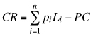
where pi is the price of lumber type i per m3, Li is the volume of lumber type i contained in one cubic meter of logs, and PC is the processing cost of one cubic meter of logs. This value can be used when log prices do not consistently reflect the value of the wood attributes (Alzamora and Apiolaza 2010). We assumed that the quality of upper sawlogs and pulplogs was well represented by market prices (MAF 2009).
Prices and shipping costs of products, as well as processing costs used to estimate log CR for appearance and structural grades have been reported by Alzamora and Apiolaza (2010), and Alzamora and Apiolaza (2013b), respectively. In summary, prices for 100x50 mm lumber were 2.5, 3.2, 4.1, 4.8 NZ$/linear m for MSG6, MSG8, MSG10 and MSG12 respectively, while the processing cost was 180 NZ$/m3.
2.3 Risk scenarios due to trait variability
GxE interaction refers to the varying effect of the environment on genotype performance. This interaction is often partitioned into changes of scale (where genotype rankings do not change) and lack of correlation that affects rankings and may lead to more complex breeding strategies (Muir et al. 1992). This paper assumes five scenarios – generated by changing tree volume, stiffness and resin defects – which act as environmental changes of scale.
Changes in volume were done by changing SED for the first log and extending that change to other logs using a linear regression resulted in updated log volumes, later aggregated to obtain new tree volumes.
Changes in stiffness were achieved by randomly choosing a log with the new required stiffness from our data set and applying that log’s outturn.
Occurrence of resin effects were modeled from a Chilean resin study that included 30 radiata pine trees with different levels of resin bleeding (Meneses and Guzmán 2003). Stems and logs were visually assessed for resin and classified in three levels: low, moderate and high resin. Logs were processed and the boards were graded twice for appearance products; the first time using regular commercial grading and the second time ignoring resin defects. The impact of resin was estimated as the board downgrading between the two assessments. These outturn downgrades were predicted using SED and resin levels for our appearance logs.
Based on the previous assumptions we defined the following variability scenarios:
- Scenario 1: The current data.
- Scenario 2: log SED increased by 10% with a corresponding increase in tree volume.
- Scenario 3: STF increased in the first, second and third logs by 10%.
- Scenario 4: volume and stiffness is increased (first log SED is increased by 25%, and 25% increase of STF for first, second and third logs).
- Scenario 5: volume is decreased (by reducing first log SED by 25%) and STF by 25%, and resin problems are introduced.
In summary, we assumed that the most undesirable events for appearance trees were to decrease volume and to suffer resin defects, while for structural trees the worst conditions were lower volume and stiffness. Variability of volume and stiffness, and resin problems occurrence have been shown to affect logs recovery value of Pinus radiata solid lumber which impose a burden for silviculturists when deciding the objective of production of a plantation (e.g. Maclaren 2002; McConchie et al. 2002; Kumar 2004; Alzamora and Apiolaza 2013b).
In addition, we incorporated variability akin to GxE lack of correlation by assuming that a randomly selected 30% of the trees stayed in the base scenario, while the remaining switched to an alternative scenario. This switch was simulated 100 times for each of the alternative scenarios, resulting in 400 extra scenarios of variability per group of trees. In addition we assumed that stiffness had no effect on the value of appearance grades, and that resin problems did not affect the value of structural products.
2.4 Portfolio analysis
The portfolio model maximized the expected return from investing in a set of trees. The model used the mean-absolute deviation of the tree returns (MAD) as the risk measure (Konno 1990; Konno and Yamazaki 1991; Konno and Koshizuka 2005). MAD models are computationally appealing, since they can be solved by using linear programming, avoiding non-convexity problems sometimes present in nonlinear models, as the Markowitz’s model. MAD models are consistent with the second degree stochastic dominance (Ogryczak and Ruszczyński 1999). Furthermore, linear programming models, as MAD, allow doing economic analyses based on dual formulation and shadow prices interpretations (Paredes and Brodie 1989).
For this application, MAD was based on different scenarios of variability on volume, stiffness and resin defects. The portfolio model was:
![]()
Subject to:

![]()
![]()
where Rij is the return of the j-th tree in the i-th scenario with j = 1,...,n and i = 1,…S; the variable xj is the fraction of the portfolio invested in the j-th tree; and, S is the total number of scenarios. Table 4 shows a summary of Rij per scenario.
Eq. 1 shows that the mean absolute deviation, represented by the term ![]() and weighted by xj, is bounded to the deviations in each scenario. The average of the deviations across scenarios (average MAD) is limited to be the maximum risk that decision makers will want to face (left side of Eq. 2). Eq. 3 shows that a weighted sum of investments in the portfolio must be equal to 1. On terms of size, the problem involves the equivalent of 41 310 trees: 3 groups (appearance, structural and appearance-structural) of 34 trees each under 405 scenarios that account for changes of scale and lack of correlation (3 x 34 x 405).
and weighted by xj, is bounded to the deviations in each scenario. The average of the deviations across scenarios (average MAD) is limited to be the maximum risk that decision makers will want to face (left side of Eq. 2). Eq. 3 shows that a weighted sum of investments in the portfolio must be equal to 1. On terms of size, the problem involves the equivalent of 41 310 trees: 3 groups (appearance, structural and appearance-structural) of 34 trees each under 405 scenarios that account for changes of scale and lack of correlation (3 x 34 x 405).
The portfolio model was modified to also analyze the selection of silvicultural regimes. In this case, the objective function maximizes the expected weighted return from investing in three silvicultural regimes, while constrains are formulated in terms of the mean absolute deviations of tree returns in each silvicultural regime. The average of deviations across trees and silvicultural regimes are limited to a maximum level of risk, which is varied to obtain an efficient frontier.
Tree returns, Rij, were annual equivalent values (NZ $/stem/year) from a cash flow including costs of establishment, silviculture and harvesting with a discount rate of 10%. Silviculture and harvesting costs were provided by New Zealand companies.
The efficient frontier was obtained by solving the linear problem for different levels of risk, identifying the maximum return portfolio for each level and plotting portfolio return versus risk. All models were run using AMPL with the CPLEX solver. Annual equivalent values changed by varying volume, stiffness and resin defects following several scenarios.
3 Results
In the first section we present the economic returns of the three groups of trees, the relationships between returns and tree attributes, as well as the return tradeoffs between volume and stiffness when allocating a tree to produce appearance and structural grades. Later we introduce the tree selections made by the portfolio model, the efficiency frontier and the trends observed when selecting silvicultural regimes.
3.1 Economic returns from trees
In the base scenario appearance trees presented a mean value of NZ $ 273/stem and NZ $ 79/m3, appearance-structural trees had a mean value of NZ $ 394/stem and NZ $ 94/m3, and structural trees showed a mean value of NZ $ 307/stem and NZ $ 79/m3.
Table 3 shows the correlations between DBH and tree values, and stiffness and tree values for the three types of trees. DBH had the highest correlation with tree value across of all trees; in contrast, the correlations between DBH and value per cubic meter of appearance-structural and structural trees were not significant (p > 0.05). Wood stiffness was highly correlated with value per cubic meter of tree; however, the correlation was not significant when using the whole tree value. These results can be explained by i- the weight of structural logs in tree value that, in average, corresponded to 53% of the tree value, and ii-the negative correlation between stiffness and volume which have been discussed in other studies (e.g. Lasserre et al. 2004; Xu and Walker 2004).
| Table 3. Pearson correlation coefficients between tree attributes and tree value. | ||
| Tree category | Diameter at breast high (DBH) | Stiffness (STF) |
| Appearance | ||
| NZ $/tree | 0.95* | |
| NZ $/m3 tree | 0.78* | |
| Appearance-structural | ||
| NZ $/tree | 0.67* | 0.17 |
| NZ $/m3 tree | –0.18 | 0.82* |
| Structural | ||
| NZ $/tree | 0.52* | 0.24 |
| NZ $/m3 tree | –0.20 | 0.82* |
| *Significant at 0.05 level. | ||
In both appearance-structural and structural trees the structural logs had the highest value per tree, which explains the high correlation between STF and the value per cubic meter of tree. However, since STF was negatively correlated with volume, the correlation between DBH and the value per cubic meter of tree was negative, although non-significant. The value contribution of non-structural logs, which are priced by volume, would preclude the significance of that correlation.
Table 4 shows the economic returns (Rij) for the three groups of trees across five scenarios of variability on volume, stiffness and resin defects. The table also shows the average value of MAD – the absolute value of the difference between the mean tree return – across five scenarios and the tree return in an individual scenario. MAD relates to risk, so a high variability or risk will be reflected in a high MAD.
| Table 4. Descriptive statistics of the average tree returns under five scenarios (Rij), and the average MAD per scenario. | |||||
| Tree groups | Scenario1 | Scenario2 | Scenario3 | Scenario4 | Scenario5 |
| Appearance | |||||
| Mean value (NZ $/tree/ year) | 0.59 | 1.02 | 0.59 | –0.62 | 1.59 |
| Maximum value | 1.88 | 2.76 | 1.88 | 0.12 | 3.92 |
| Minimum value | –0.30 | –0.16 | –0.30 | –1.44 | 0.04 |
| MAD | 0.07 | 0.39 | 0.07 | 1.25 | 0.95 |
| Appearance-structural | |||||
| Mean value (NZ $/tree/ year) | 1.22 | 1.66 | 2.26 | –0.46 | 4.62 |
| Maximum value | 2.58 | 3.21 | 3.77 | –0.05 | 7.67 |
| Minimum value | –0.15 | –0.17 | 0.07 | –0.71 | 1.88 |
| MAD | 0.64 | 0.30 | 0.57 | 2.32 | 2.76 |
| Structural | |||||
| Mean value (NZ $/tree/ year) | 0.76 | 1.06 | 1.75 | –0.44 | 4.57 |
| Maximum value | 2.94 | 3.76 | 3.59 | –0.08 | 8.31 |
| Minimum value | –1.76 | –1.97 | –0.07 | –1.18 | 0.93 |
| MAD | 0.78 | 0.49 | 0.27 | 1.98 | 3.03 |
In the base scenario, appearance-structural trees had the highest mean gross return whereas appearance trees had the lowest one. The mean gross returns of structural trees were between the two previous groups. Return and risk had their lowest value for appearance trees while structural trees had the highest MAD; nevertheless, the returns of appearance-structural and structural trees were similar with non-significant differences in the base scenario (p > 0.05).
Tree-return trends observed in the base scenario were maintained across all alternatives; however, returns from structural trees were slightly superior to those from appearance-structural trees in the optimistic scenario. This was expected because a simultaneous increase of volume and stiffness implied that every log of the structural trees increased its value while for the appearance-structural trees only the first log increased its value due to extra volume. In general, trees that produced appearance lumber had a proportionally higher value increase when increasing volume than when improving stiffness. In contrast, those trees that generated structural grades had their highest value increase when improving stiffness. The trends for risk/MAD were different; in the base scenario, structural trees had the highest MAD, appearance trees the lowest MAD and appearance-structural trees an intermediate value. In the second scenario (volume increase), the highest MAD was for appearance trees and lowest for the appearance-structural trees. Nevertheless, for both the third scenario of STF increase, and the fourth negative scenario, MAD had the highest value for appearance-structural trees. Finally, in the positive scenario, structural trees obtained the highest MAD. In summary, although appearance-structural and structural trees had similar gross returns; the latter presented the highest variability, in 3 out of the 5 scenarios, making them the riskiest assets. This result was mainly due to the dependence of structural trees value on stiffness, which had a high variability (see Table 1).
There were value tradeoffs when allocating trees to produce appearance and structural grades. Table 5 presents the value increase (%) of logs and trees, when increasing volume or stiffness while maintaining the other traits unchanged. This tradeoff between volume and stiffness would also contribute to explain that appearance-structural trees presented MAD values lower than structural trees across scenarios of variability.
| Table 5. Value increase on logs and trees due to volume and stiffness increase. | |||
| Appearance | Appearance-structural | Structural | |
| Volume increase | |||
| Butt log | 31% | 17% | 21% |
| Second log | 32% | 22% | 22% |
| Third log | 31% | 23% | 23% |
| Tree | 29% | 19% | 22% |
| Stiffness increase | |||
| Butt log | 0% | 0% | 71% |
| Second log | 0% | 58% | 58% |
| Third log | 0% | 81% | 81% |
| Tree | 0% | 32% | 52% |
The pruned log index (PLI) of appearance-structural trees increased from 6.7 to 7.0 and the log value increased by 17% when increasing tree volume. The second and third structural logs increased by 22 and 23%, respectively, and the tree value increased by 19%. However, these values are lower than those achieved by trees with a single production goal. Similarly, when increasing stiffness by 10%, structural trees achieved the highest values; however, those logs and trees that produce appearance grades did not change their values.
Appearance-structural trees displayed intermediate positions when increasing volume or stiffness, with proportionally lower value increases compared to trees with a single production goal. The intermediate position of these trees is also explained by the tradeoff between stiffness and growth (Lasserre et al. 2004; Watt et al. 2005; Waghorn et al. 2007b). Increasing only volume decreases average wood stiffness because there is a larger proportion of corewood. The increase of value for unpruned logs is proportionally lower than that for butt logs, because their value is more dependent on stiffness than on volume. On the other hand, this tradeoff would tend to match the values of the butt log for appearance grades and the unpruned logs for structural purposes. This effect could be advantageous from a portfolio perspective, since it favors assets with high return and low variability.
3.2 Portfolio selection of trees
There were eleven trees in the general solution for the five scenarios of gross tree returns described in Table 5: 55% appearance, 27% appearance-structural and 18% structural. Under high levels of risk (MAD > 2.9) the model selected only structural trees. As risk decreased so did the mean gross return, and the model selected an increasing number of appearance-structural trees. The solution considered only appearance-structural trees for MAD between 1.3–0.95. The model apportioned the investment between appearance and appearance-structural trees for MAD lower than 0.9.
When considering the extra GxE scenarios that were integrated in the portfolio model, the solution included six appearance (60%), two appearance-structural (20%) and two structural trees (20%). Despite the additional variability, the selections were similar to those for only 5 scenarios. The model selected a structural tree for high variability, but as the risk decreased appearance-structural and an additional structural trees were selected. Appearance-structural trees were selected in a small range of risk; in contrast, appearance trees were chosen across of a broad range of risk (MAD between 1 and 0.28).
For returns discounting silvicultural and harvesting costs both basic 5 and extra 400 (GxE) scenarios generated similar trends. There were twelve trees in the solution: 66% appearance (8, 22, 23, 25, 28, 30, 31, 34), 17% appearance-structural (48 and 55) and 17% structural (81 and 86). Fig. 1 presents the proportion for selected trees under changing risk. The model selected only one structural tree (86) for MAD between 5 and 1.8. Further decreasing MAD and returns, the model diversified by including another structural and some appearance-structural trees. The model apportioned the investment into three types of trees as MAD decreased from 1.5 to 1.0 and selected only appearance trees for MAD lower than 1. This suggests that, under the assumed circumstances, appearance trees would be the best option for risk adverse decision makers.
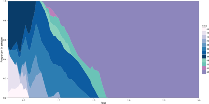
Fig. 1. Proportion of trees selected in the solution for different levels of risk. The solutions include appearance (8, 22, 23, 25, 28, 30, 31, 34, blue palette), appearance-structural (48 and 55, green palette) and structural (81 and 86, purple palette) trees.
Table 6 presents basic characteristics for five trees included in the solution which had the highest weight in the selection for each tree group. While there were eight appearance trees in the solution, we only present the tree with the highest participation in order to simplify the discussion. Structural trees presented the lowest DBH and the highest stiffness. In addition, their second and third logs had the highest ratio between stiffness and small end diameter (higher than 1: 4), which would suggest high productive efficiency for structural lumber. Similar results were reported by Alzamora and Apiolaza (2013a) when using a non-parametric efficiency analysis to characterize the most efficient logs to produce New Zealand structural grades. Furthermore, structural logs from trees 81 and 86 were included in the group of most efficient logs.
| Table 6. Characteristics of the five trees selected in the portfolio analysis. | |||||||||
| Tree DBH (cm) | Butt log SED (cm) | 2nd log SED (cm) | 3rd log SED (cm) | 1st log STF (GPa) | 2nd log STF (GPa) | 3rd log STF (GPa) | 2nd log STF/SED | 3rd log STF/SED | |
| Structural trees | |||||||||
| Tree 86 | 55.3 | 44.4 | 40.8 | 36.2 | 9.91 | 11.6 | 10.6 | 0.28 | 0.29 |
| Tree 81 | 56.5 | 41.8 | 36.4 | 31.7 | 7.11 | 9.5 | 8.5 | 0.26 | 0.28 |
| Appearance-structural trees | |||||||||
| Tree DBH (cm) | Butt log SED (cm) | 2nd log SED (cm) | 3rd log SED (cm) | 1st log PLI | 2nd log STF (GPa) | 3rd log STF (GPa) | 2nd log STF/SED | 3rd log STF/SED | |
| Tree 55 | 56.7 | 48.2 | 43.3 | 39.8 | 6.7 | 9.1 | 8.9 | 0.21 | 0.22 |
| Tree 48 | 75.9 | 60.4 | 56.3 | 50.6 | 7.3 | 7.9 | 8.0 | 0.14 | 0.16 |
| Appearance trees | |||||||||
| Tree DBH (cm) | Butt log SED (cm) | 2nd log SED (cm) | 3rd log SED (cm) | 1st log PLI | 2nd log MIL (cm) | 3rd log MIL (cm) | 2nd log BIL (cm) | 3rd log BIL (cm) | |
| Tree 34 | 58.0 | 46.5 | 43.5 | 38.9 | 6.3 | 189 | 83 | 179 | 112 |
Appearance-structural trees had high quality butt logs, represented by their SED and PLI; however, their unpruned logs had lower quality, with a low STF: SED ratio by comparison with structural trees. This suggests that those trees were selected mostly due to the quality and value of their butt log. Although most second and third logs had STF greater than 8 GPa, their STF: SED ratios were lower than for structural trees. The strength of appearance-structural would be mainly based on the first pruned log and its traits. Appearance trees had DBH greater that 56 cm, a PLI greater than 5, and a medium internode length (MIL) greater than 35 cm.
Fig. 2 depicts the efficiency frontier derived from the selected trees. The points correspond to the portfolios that have the highest possible expected return for a given level of risk. There was a wide range of risk with constant return, corresponding to a single structural tree (86) selected, illustrating the tradeoff between return and risk. The high returns from a single tree compensated the variability (MAD 3.64) for a wide-range of risk.
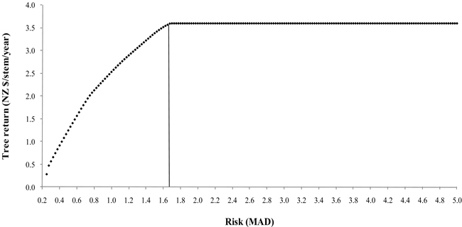
Fig. 2. Portfolio efficiency frontier for the selected trees.
3.3 Portfolio selection of silvicultural regimes
The portfolio model generated different results for 5 (GxE with only changes of scale) or 405 (GxE with changes of scale and lack of correlation) scenarios of trait variability when analyzing the risk-return tradeoff between groups of trees. Using 405 scenarios (i.e. accounting for lack of correlation) and allowing for a high variability of returns (MAD > 1.5), the model selected the regime to produce both appearance and structural lumber. As the risk declined the model also selected the structural regime but in a very narrow range of risk (MAD: 1.38–1.3). The model apportioned between appearance-structural and appearance regimes for MAD lower than 1.3; however, only the appearance regime was selected for risk aversion criteria (MAD < 0.7). The portfolio model did not select the structural regime when using only the first five variability scenarios. Instead, the model selected an appearance and structural grades regime for high risk and an appearance regime for low risk (MAD < 1).
4 Discussion
Portfolio theory has been used in animal and crop breeding, although its main applications have been on (i) dealing with the tradeoff between genetic merit and variance of the predicted genetic value and (ii) mazimizing genetic gain subject to diversity constraints (e.g. Schneeberger et al. 1982; Galligan et al. 1991; Nash and Rogers 1996; Danusevicius and Lindgren 2008). In our experience with radiata pine, neither the variability of predicted error variances nor genetic diversity constraints are problematic enough to warrant major efforts on their control. In contrast, performance instability due to environmental change and (potentially) market changes present larger risks that merit attention. That is, we have approached risk as variability of breeding objective traits that, in turn, affect the quantity and quality of appearance and structural lumber produced by the deployment units (Jayawickrama 2001; McConchie and Turner 2002; Xu and Walker 2004; Apiolaza 2009; Alzamora and Apiolaza 2010). Tree return analyses supported the importance of these traits; thus, trees for appearance lumber obtained their highest value recovery from the butt pruned log, which had the biggest volume and the longest defect free pieces. In the case of structural trees, second and third logs were the most valuable (53% of tree value) because they had the highest stiffness of the tree, which has been reported by other studies (e.g. Xu and Walker 2004; Ivković et al. 2006).
The negative correlation between stiffness and volume supports the results reported by other researchers (e.g. Lasserre et al. 2004; Xu and Walker 2004). However, there would be a defined relative participation of volume and stiffness in a log that results in a high recovery of structural grades. The best structural tree presented a high ratio between stiffness and small end diameter (higher than 1: 4) in its structural logs, which resulted in a high recovery of structural grades. Similar results were reported by Alzamora and Apiolaza (2013b) and Alzamora (2010) when using efficiency frontiers to characterize the most efficient logs to produce New Zealand structural grades.
Appearance-structural trees had the highest return in the current scenario; however, structural trees were the most profitable when increasing volume and stiffness. These trees showed a high variability in stiffness (see Table 1) and returns (see Table 5) which suggested that using genetically improved material (such as clones) for stiffness could be a good investment to reduce the risk of variable returns. The advantages of radiata pine clonal forestry has been discussed by Burdon (2001), Sorensson (2002), and Burdon and Aimers-Halliday (2003).
Appearance trees had their highest returns when increasing volume, which suggests that combining an efficient silviculture with genetically improved material for growth would achieve a high value recovery in appearance products (Meneses and Guzmán 2000). Appearance trees are not usually grown due to the low recovery of appearance grades from the unpruned logs due to short internodes; however, trees of this study had a MIL greater than 58 cm that makes this scenario comparable to having material genetically improved for internode length.
Nevertheless, to produce appearance and structural grades from a single tree the alternatives are making stocking decisions to minimize the tradeoff between volume and stiffness, or planting improved material for stiffness. The economic benefits of increasing stiffness, particularly in corewood, have been stressed by Dickson and Walker (1997).
The portfolio model selected a structural tree for high variability, but as the risk decreased appearance-structural and an additional structural trees were selected. Appearance-structural trees were selected in a small range of risk; in contrast, appearance trees were chosen across of a broad range of risk. Furthermore, under low variability (risk), portfolio selected only appearance trees. Thus, under the assumed circumstances, these trees would be the best option for risk adverse decision makers. This results from volume increases favoring all tree logs; in the same way, resin defects affect each sawn log. Thus, there would not be tradeoffs affecting returns variability; in addition, resin problems had comparatively less impact in these trees than stiffness reductions for structural trees.
The portfolio model used in this study was appropriate, as tree returns presented a normal distribution; however, MAD is a symmetric risk measure, which implies that it does not differentiate between the desirable upside and undesirable downside risks (Wu, Yue, and Wang 2005). Future studies should contrast the selections made by using this model with those based on downside risk measures such as the Value at Risk and the Conditional Value at Risk (Konno and Yamazaki 1991; Konno and Koshizuka 2005).
We deliberately did not include variability of product prices in this research, as preliminary analyses showed a high correlation between products prices among years. Accordingly, the current trend of allocating the highest prices to long defect-free pieces for appearance use, and the lumber with the highest machine stress grade for structural use, seems a reasonable assumption for future conditions. This assumption let us isolate the impact of wood-trait variability on tree selection from a financial point of view. Furthermore, our results should be considered as a case study outlining the process faced by firms breeding and multiplying deployment units. As such, the results will not necessarily apply to all firms working with radiata pine, but the general model will provide a useful starting point for specific decisions.
5 Conclusions
Trees from three silvicultural regimes were approached as an investment problem with a tradeoff between returns and risk. The analysis permitted selecting and characterizing the most robust trees from an investment point of view.
Producing appearance and structural grades from a tree had a stabilizing effect on returns, as there are phenotypic tradeoffs between stiffness and volume under optimistic and pessimistic growing scenarios. These trees had a lower variability than structural trees; although both groups of trees had similar returns.
The regime for appearance-structural trees was selected across a wide range of risk when modeling a portfolio to select silvicultural regimes. This showed the benefits of product diversification at the tree level.
Trees to produce appearance grades had the lowest values for return and risk; as a result they were selected under high risk aversion.
The high returns and variability displayed by structural trees suggests an opportunity for narrowing genetic variability (via clonal or family forestry) to make the returns from radiata pine structural grades lumber less risky.
This risk approach could be improved by adding information of product prices, discount rates and production costs to better represent the risk involved in the forestry business.
References
Alzamora R.M. (2010). Valuing breeding traits for appearance and structural timber in radiata pine. PhD Thesis, University of Canterbury. http://ir.canterbury.ac.nz/handle/10092/5077.
Alzamora R.M., Apiolaza L.A. (2010). A hedonic approach to value Pinus radiata log traits for appearance-grade lumber production. Forest Science 53: 283–291.
Alzamora, R.M., Apiolaza, L.A. (2013a). A DEA approach to assess the efficiency of radiata pine logs to produce New Zealand structural grades. Journal of Forest Economics.
Alzamora R.M., Apiolaza L.A. (2013b). Using a production approach to estimate economic weights for structural attributes of Pinus radiata wood. Scandinavian Journal of Forest Research 28: 282–290.
Apiolaza L.A. (2009). Very early selection for solid wood quality: screening for early winners. Annals of Forest Science 66: 601–611.
Apiolaza L.A. (2011). Basic density of radiata pine in New Zealand: genetic and environmental factors. Tree Genetics and Genomes. doi: 10.1007/s11295-011-0423-1.
Barkley A., Peterson H.H. (2008). Wheat variety selection: an application of portfolio theory to improve returns. Proceedings of the NCCC-134 Conference on Applied Commodity Price Analysis, Forecasting, and Market Risk Management, 21–22 April, St. Louis MO, USA. http://www.farmdoc.uiuc.edu/nccc134. [Cited 4 April 2011].
Bascuñán A., Moore J.R., Walker J.C.F. (2006). Variations in the dynamic modulus of elasticity with proximity to the stand edge in radiata pine stands on the Canterbury Plains, New Zealand. New Zealand Journal of Forestry 51: 4–8.
Bruce D., Curtis R.O., Vancoevering C. (1968). Development of a system of taper and volume tables for red alder. Forest Science 14: 339–350.
Burdon R.D. (2001). Genetic aspects of risk-species diversification, genetic management and genetic engineering. New Zealand Journal of Forestry 45: 20–24.
Burdon R.D., Aimers-Halliday J. (2003). Risk management for clonal forestry with Pinus radiata – analysis and review. 1: Strategic issues and risk spread. New Zealand Journal of Forestry Science 33: 156–180.
Byrne P., Lee S. (1997). Real estate portfolio analysis under conditions of non-normality: the case of NCREIF. The Journal of Real Estate Portfolio Management 3: 37–46.
Chauhan S.S., Donnelly R., Huang C.L., Nakada R., Yafang Y., Walker J.C.F. (2006a). Wood quality: multifaceted opportunities. In: Walker J.C.F. (ed.). Primary wood processing, principles and practice. 2nd edition. Springer p. 121–158.
Chauhan S.S., Donnelly R., Huang C.L., Nakada R., Yafang Y., Walker J.C.F. (2006b). Wood quality: multifaceted opportunities. In: Walker J.C.F. (ed.). Primary wood processing, principles and practice. 2nd edition. Springer. p. 159–202.
Clutter M., Mendell B., Newman D., Wear D., Greis J. (2005). Strategic factors driving timberland ownership changes in the U.S. south. http://www.srs.fs.usda.gov/econ/pubs/southernmarkets/strategic-factors-and-ownership-v1.pdf. [Cited 6 May 2010].
Cown D.J. (1973). Resin pockets: their occurrence and formation in New Zealand forests. New Zealand Journal of Forestry 18: 233–251.
Crowe K.A., Parker W.H. (2008). Using portfolio theory to guide reforestation and restoration under climate change scenarios. Climatic Change 89: 355–370.
Danusevicius D., Lindgren D. (2008). Strategies for optimal deployment of related clones into seed orchards. Silvae Genetica 57: 119–127.
Daniels P.W., Helms U.E., Baker F.S. (1979). Principles of silviculture. Mc-Graw-Hill.
Davis L.S., Johnson K.N. (1987). Forest management. McGraw-Hill, New York.
Dickson R.L., Walker J.C.F. (1997). Growing commodities or designer trees. Commonwealth Forestry Review 76: 273–279.
Dunham R.A., Cameron A.D. (2000). Crown, stem and wood properties of wind-damaged and undamaged Sitka spruce. Forest Ecology and Management 135: 73–81.
Emms G.W., Jones T.G., McKinley R., Gaunt D., Cown D., McConchie D., Andrews M. (2008). Influence of knot size and density and stiffness profiles on stiffness grade out-turn prediction from log acoustic velocity. WQI Report STR27. 77 p.
Jones T.G., Emms G.W. (2010). Influence of acoustic velocity, density, and knots on the stiffness grade outturn of radiata pine logs. Wood and Fiber Science 42: 1–9.
Evans R., Ilic J. (2001). Rapid prediction of wood stiffness from microfibril angle and density. Forest Products Journal 51: 53–57.
Galligan D.T., Ramberg C., Curtis C., Ferguson J., Fetrow J. (1991). Application of portfolio theory in decision tree analysis. Journal of Dairy Science 74: 2138–2144.
Gapare W.J., Ivković M., Baltunis B.S., Matheson A.C., Wu H.X. (2009). Genetic stability of wood density and diameter in Pinus radiata D. Don plantation estate across Australia. Tree Genetics and Genomes 6: 113–125.
Heikkinen V.P. (2002). Co-integration of timber and financial markets – implications for portfolio selection. Forest Science 48: 118–128.
Heikkinen V.P. (2003). Timber harvesting as a part of the portfolio management: a multiperiod stochastic optimisation approach. Management Science 49: 131–142.
Ivković M., Wu H.X., McRae T.A., Powell M.B. (2006). Developing breeding objectives for radiata pine structural wood production. I. Bioeconomic model and economic weights. Canadian Journal of Forest Research 36: 2920–2931.
Johnson G.R., Burdon R.D.1990. Family-site interaction in Pinus radiata: implications for progeny testing strategy and regionalised breeding in New Zealand. Silvae Genetica 39: 55–62.
Konno H. (1990). Piecewise linear risk function and portfolio optimization. Journal of the Operations Research Society of Japan 33: 139–156.
Konno H., Koshizuka T. (2005). Mean-absolute deviation model. IIE Transactions 37: 893–900.
Konno H., Yamazaki H. (1991). Mean-absolute deviation portfolio optimization model and its applications to Tokyo stock market. Management Science 37: 519–531.
Korol R.L., Kirschbaum M.U.F, Farquhar G.D., Jeffreys M. (1999). Effects of water status and soil fertility on the C-isotope signature in Pinus radiata. Tree Physiology 19: 551–562.
Kumar S. (2004). Genetic parameter estimates for wood stiffness, strength, internal checking, and resin bleeding for radiata pine. Canadian Journal of Forest Research 34: 2601–2610.
Lasserre J.P., Mason E.G., Watt M.S. (2004). The influence of initial stocking on corewood stiffness in a clonal experiment of 11 year-old Pinus radiata D. Don. New Zealand Journal of Forestry 49: 18–23.
Lindstrom H., Evans R., Reale. M. (2005). Implications of selecting tree clones with high modulus of elasticity. New Zealand Journal of Forestry Science 35: 50–71.
Maclaren P. (1993). Radiata pine growers’ manual. New Zealand Forest Research Institute (FRI) Bulletin 184. 140 p.
Maclaren P. (2002). Internal wood quality of radiata pine on farm sites – a review of the issues. New Zealand Journal of Forestry, November: 24–28.
Markowitz H. (1952). Portfolio selection. The Journal of Finance 7: 77–91.
Matheson A.C., Wu H.X. (2005). Genotype by environment interactions in an Australia-wide radiata pine diallel mating experiment: implications for regionalized breeding. Forest Science 51: 29–40.
McConchie D., Turner J., McKinley R., Young G., Treloar C. (2002). The relationship between external resinous characteristics on pruned butt logs and clearwood grade recovery. New Zealand Forest Research Institute, Rotorua. WQ Internal Report 9500.
Meneses M.O., Guzmán S. (2000). Análisis de la eficiencia de la silvicultura destinada a la obtención de madera libre de nudos en plantaciones de pino radiata en Chile. Bosque 21: 85–93.
Meneses M.O., Guzmán S. (2003). Clasificación de rollizos y rodales. Informe N° 5 Proposición de un sistema de clasificación de trozas podadas y no podadas. Universidad Austral de Chile, Valdivia, Chile. 178 p.
Muir W., Nyquist W.E., Xu S. (1992). Alternative partitioning of the genotype-by-environment interaction. Theoretical and Applied Genetics 84: 193–200.
Mills Jr W.L., Hoover W.L. (1982). Investment in forest land: aspects of risk and diversification. Land Economics 58: 33–51.
Nalley L. Barkley A., Brad W., Hignight J. (2009). Enhancing farm profitability through portfolio analysis: the case of spatial rice variety selection. Journal of Agricultural & Applied Economics 41: 641–652.
Nambiar E.K.S. (1995). Relationships between water, nutrients and productivity in Australian forests: application to wood production and quality. Plant and Soil 168: 427–435.
Nash D.L., Rogers G.W. (1996). Risk management in herd sire portfolio selection: a comparison of rounded quadratic and separable convex programming. Journal of Dairy Science 79: 301–309.
Neuner S., Beinhofer B., Knoke T. (2013). The optimal tree species composition for a private forest enterprise – applying the theory of portfolio selection. Scandinavian Journal of Forest Research 28: 38–48.
Ogryczak W., Ruszczyński A. (1999). Theory and methodology: from stochastic dominance to mean-risk models: semideviations as risk measures. European Journal of Operational Research 116: 33–50.
Ormerod D.W. (1973). A simple bole model. The Forestry Chronicle 49: 136–138.
Paredes G., Brodie D. (1989). Land value and the linkage between stand and forest level analyses. Land Economics 65: 158–166.
Park J.C. (1989). Pruned log index. New Zealand Journal of Forestry Science 19: 41–53.
Pruyn M.L., Ewers B.J., Telewski F.W. (2000). Thigmomorphogenesis: changes in the morphology and mechanical properties of two Populus hybrids in response to mechanical perturbation. Tree Physiology 20: 535–540.
Raymond C.A. (2011). Genotype by environment interactions for Pinus radiata in New South Wales, Australia. Tree Genetics and Genomes. doi: 10.1007/s11295-011-0376-4.
Ruszczynski A., Vanderbei R.J. (2003). Frontiers of stochastically nondominated portfolios. Econometrica 71: 1287–1297.
Schneeberger M., Freeman A.E., Boehlje M.D. (1982). Application of portfolio theory to dairy sire selection. Journal of Dairy Science 65: 404–409.
Shapcott J. (1992). Index tracking: genetic algorithms for investment portfolio selection. Edinburgh Parallel Computing Centre Technical Report EPCC-SS92-24. 25 p. http://www.smartquant.com/references/PortfolioSelection/portfselect2.pdf. [Cited 4 April 2011].
Sharpe W.F. (1971). A linear programming approximation for the general portfolio analysis problem. Journal of Financial and Quantitative Analysis 6: 1263–1275.
Smith S.P., Hammond K. (1987). Portfolio theory, utility theory and mate selection. Genetics Selection Evolution 19: 321–336.
Sorensson C. (2002). Reflections on radiata pine genetic improvement by a clonal forester. New Zealand Journal of Forestry 47: 29–31.
Stone B.K. (2009). A linear programming formulation of the general portfolio selection problem. Journal of Financial and Quantitative Analysis 8: 621–636.
Telewski F.W., Jaffe M.J. (1986). Thigmomorphogenesis: field and laboratory studies of Abies fraseri in response to wind or mechanical perturbation. Physiologia Plantarum 66: 211–218.
Todoroki C.L., Carson S.D. (2003). Managing the future forest resource through designer trees. International Transactions in Operational Research 10: 449–460.
Tsehaye A. (1995). Within- and between-tree variations in the wood quality of radiata pine. Ph.D. Thesis. University of Canterbury Christchurch, New Zealand. 264 p.
WWPA. (1989). Western wood species book Vol.3: Factory lumber. Western Wood Products Association, Oregon, USA. http: //www2.wwpa.org. [Cited 4 April 2011].
Waghorn M.J., Mason E.G., Watt M.S. (2007a). Influence of initial stand density and genotype on longitudinal variation in modulus of elasticity for 17-year-old Pinus radiata. Forest Ecology and Management 252: 67–72.
Waghorn M.J., Watt M.S., Mason E.G. (2007b). Influence of tree morphology, genetics, and initial stand density on outerwood modulus of elasticity of 17-year-old Pinus radiata. Forest Ecology and Management 244: 86–92.
Walford GB (1985) The mechanical properties of New Zealand-grown radiata pine for export to Australia. FRI Bulletin 93. 27 p.
Watt M.S., Downes G.M., Jones T., Ottenschlaeger M., Leckie A.C., Smaill S.J., Kimberley M.O., Brownlie R. (2009). Effect of stem guying on the incidence of resin pockets. Forest Ecology and Management 258: 1913–1917.
Weng Y., Park Y.S., Krasowski M.J. (2010). Managing genetic gain and diversity in clonal deployment of white spruce in New Brunswick, Canada. Tree Genetics and Genomes 6: 367–376.
Woollons R., Manley B., Park J. (2008). Factors influencing the formation of resin pockets in pruned radiata pine butt logs in New Zealand. New Zealand Journal of Forestry Science 38: 323–333.
Xu P., Walker J.C.F. (2004). Stiffness gradients in radiata pine trees. Wood Science and Technology 38: 1–9.
Zhang S.Y., Chauret G., Ren H.Q., Desjardins R. (2002). Impact of initial spacing on plantation black spruce lumber grade yield, bending properties, and MSR yield. Wood and Fiber Science 34: 460–475.
Zinkhan F.C. (1988). Forestry projects, modern portfolio theory, and discount rate selection. Southern Journal of Applied Forestry 12: 132–135.
Zobel B.J., Van Buijtenen J.P. (1989). Wood variation: its causes and control. Springer, Berlin.
Total of 78 references
