Rene Zamora-Cristales  ,
Kevin Boston,
John Sessions,
Glen Murphy
,
Kevin Boston,
John Sessions,
Glen Murphy
Stochastic simulation and optimization of mobile chipping economics in processing and transport of forest biomass from residues
Zamora-Cristales R., Boston K., Sessions J., Murphy G. (2013). Stochastic simulation and optimization of mobile chipping economics in processing and transport of forest biomass from residues. Silva Fennica vol. 47 no. 5 article id 937. https://doi.org/10.14214/sf.937
Highlights
- A stochastic simulation model is proposed to analyze forest biomass operations
- The cost of chipper and truck waiting times was estimated in forest biomass recovery operations
- The economic effect of truck-machine interactions under uncertainty was analyzed
- Road characteristics and processing location have an economic impact in truck and chipper waiting times
Abstract
We analyzed the economics of mobile chipping and transport of biomass from forest residues for energy purposes under uncertainty. A discrete-event simulation model was developed and utilized to quantify the impacts of controllable and environmental variables on productivity in order to determine the most cost effective transportation options under steep terrain conditions. Truck-chipper interactions were analyzed to show their effect on truck and chipper standing time. A costing model was developed to account for operating and standing time cost (for the chipper and trucks). The model used information from time studies of each activity in the productive cycle and spatial-temporal information obtained from geographic information system (GIS) devices, and tracking analysis of machine and truck movements. The model was validated in field operations, and proved to be accurate in providing the expected productivity. A cost distribution was elaborated to support operational decisions of forest managers, landowners and risk-averse contractors. Different scenarios were developed to illustrate the economic effects due to changes in road characteristics such as in-highway transport distance, in-forest internal road distance and pile to trailer chipper traveling distances.
Keywords
forest planning;
simulation;
optimization;
economics;
decision analysis;
forest biomass;
renewable energy
-
Zamora-Cristales,
Department of Forest Engineering, Resources, and Management, College of Forestry, Oregon State University, 280 Peavy Hall, Corvallis, OR 97331, USA
E-mail
rene.zamora@oregonstate.edu
- Boston, Department of Forest Engineering, Resources, and Management, College of Forestry, Oregon State University, 280 Peavy Hall, Corvallis, OR 97331, USA E-mail kevin.boston@oregonstate.edu
- Sessions, Department of Forest Engineering, Resources, and Management, College of Forestry, Oregon State University, 280 Peavy Hall, Corvallis, OR 97331, USA E-mail john.sessions@oregonstate.edu
- Murphy, Waiariki Institute of Technology, Rotorua, New Zealand E-mail glen.murphy@waiariki.ac.nz
Received 12 June 2013 Accepted 4 November 2013 Published 31 December 2013
Views 104650
Available at https://doi.org/10.14214/sf.937 | Download PDF

Supplementary Files
1 Introduction
Forest residues, created as a byproduct of logging operations, are a renewable resource that can be used for electricity generation. These residues also have the potential to produce liquid fuels although conversion procedures are still experimental. In 2011, the Northwest Advanced Renewables Alliance (NARA), a group of US public universities, government laboratories and private industry was formed to build a sustainable supply chain for aviation fuel from forest and mill residues, municipal solid waste and energy forest crops (NARA 2011).
Forest residues consist of branches, tops, breakage, defect, and trees not meeting utilization specifications for timber and pulp (paper production). One of the most important distinctions of the use of forest residues for energy purposes, is that they are not currently used for other commercial purposes and do not compete with human food supply chains. Fuels derived from forest residues from non-federal lands and certain federal lands qualify as renewable energy sources under the current US Renewable Fuel Standard (Bracemort 2012).
After timber harvesting, most of the forest residues are piled and burned to clean the areas for replanting, and to reduce fuel loadings, and potential insect and rodent problems. It is estimated that a total of 127.4 million m3 of logging residues were produced in the United States in 2006 (Smith et al. 2009).
To economically handle and transport forest residues, biomass has to be mechanically reduced in particle size (comminution). This process reduces the heterogeneous composition of the material and facilitates the handling and delivery process (Hakkila 1989). Residues can be processed using chippers or grinders (Staudhammer et al. 2011). In the US, after comminution, processed residues are transported using chips-vans.
The use of a mobile chipper for processing forest residues for energy purposes represents an alternative to the use of stationary grinding machines currently used in the U.S. Pacific Northwest. The advantages of mobile chippers are the mobility to reach different locations within the forest where the forest residue piles remain following harvesting, flexibility to unload the material into different types of containers and a self-feeding system. Also the use of independent containers partially disconnects processing from trucking reducing truck dependence. However productivity is highly sensitive to the size, cleanness and type of harvest residue material, and the number of stages involved in the chipping process (chipping, moving, and dumping into trailers) gives more complexity to this process compared with stationary equipment. Consequently, uncertainties might arise at each stage of the process and can have a significant effect in the overall productivity. Uncertainty in this paper is analyzed in non-controllable factors that are usually environmental variables in which the decisions are not in control of the operator or planner (Taguchi 1987). Examples of these variables in mobile chipping include the size, shape and location of the forest residue piles, degree of heterogeneity of the material within the pile, machine driving speed between the piles due to terrain and maneuverability conditions and interactions between trucks and machine-truck.
Biomass from forest residues is a low value product in the forest supply chain. Processing in the field requires the use of expensive machinery with usually high fixed costs. Transportation costs are highly dependent on the travel time between the forest unit and the plant and the moisture content and bulk density of the processed residues. Given the reduced marginal income of this operation, efficient planning and cost management is needed to ensure the long term success of this emerging renewable source of energy. A careful analysis of each operational stage is necessary to understand the elements that affect productivity and consequent profitability of the operation. Due to the low margin of profit of this operation, sources of uncertainty need to be understood to produce an accurate estimation of the net profit variability and to support the decision process for forest managers, landowners and risk adverse contractors. At the operational level optimization is necessary to determine the most cost-effective transportation option given the chipper productivity, road and landing access and residue assortment.
In mobile chipping, equipment balancing can be an issue if there is not sufficient availability of trucks to replace the trailers in the forest. Truck-chipper interactions occur when the behavior of trucks (e.g. truck inter-arrival times) affect chipper productivity increasing standing times. Spinelli and Visser (2009) describe this type of truck-machine interference as part of organizational delays. If there are not available trailers to unload the chipper bin, then the chipper has to wait until a truck arrives and places an empty trailer on the landing. Similarly, if the trailer is not full with chips when a truck arrives to the site, then the truck has to wait until the trailer is full. Truck interference can also occur due to single lane passage and limited turn-around locations. Therefore, if a truck arrives to the site and a second truck is still in the chipping area, then the truck that is arriving must wait further down the road until the other truck passes the point where the first truck is waiting. Additionally the variability on productivity of the mobile chipper adds complexity to the problem. Adding more reserve trailers to reduce chipper dependence on the trucks is often not a feasible option due to the limited available space in forest roads under steep slope conditions to locate the trailers.
Simulation has been used in forest operations for many years to analyze systems design and performance although more deterministic models exist due to the complexity in the analysis of random variations. Bradley et al. (1975) designed a computer simulator for full tree chipping and trucking. Machine interactions between skidders, feller bunchers chipper and truck were analyzed. Asikainen (2010) simulated the stump crushing and truck transport of chips in northern Europe. The number of optimal trucks needed for the stump crushing operation was estimated based on the distance from the forest to the heating plant. Author concluded that in energy supply chains, strong interactions of random elements can affect system balancing. Baumgrass et al. (1993) discussed the use of simulation to estimate and validate harvest production. Although their paper did not specifically mention the use of simulation in forest biomass recovery operations, it described how simulation can be a useful method to analyze relationships and effect of different equipment in forest operations. In relation to forest biomass collection, Gallis (1995) simulated a forest biomass harvesting and transportation system in Greece using activity oriented stochastic simulation. Also no details were provided about the costing process that was used to evaluate the operations. Additionally no information about the robustness or validity of the probability density functions is reported and the simulation system did not account for standing times related to equipment balancing. Mobini et al. (2011) developed a discrete-event simulation model to evaluate the biomass delivery cost to a potential power plant. The authors discussed several processing and transportation systems at the tactical level but no details are giving about the effect of truck-machine interactions or road access on productivity. The variability of productivity was analyzed as an overall system not segregated into different operational stages. Little information is given about the productivity distributions used within the study and its applicability to other processing systems such as mobile chipping. MacDonagh et al. (2004) developed two simulation systems to analyze forest harvesting operations. The author also discussed the impact of machine interactions on productivity of the system, however the study is not directly related to biomass recovery operations and no methodology is developed in relation to machine and trucks standing cost. Talbot and Suadicani (2005) developed a deterministic simulation model to analyze in-field chipping and extraction systems in spruce thinnings. They discussed strategies for decoupling the chipping operation from bin forwarding to maximize chipper productivity. Although the cost of chipper bin forwarder interactions is accounted for in the study, few details are giving about the effect of truck configuration and road accessibility on chipping performance and truck-machine interactions
The main goal of this study is to improve the efficiency of the forest biomass supply by minimizing mobile chipping processing and transportation costs at the operational level under uncertainty. Processing and transportation costs include the mobile chipper and tractor–trailer variable and fixed cost, the mobilization cost to transport the machinery between different forest units and the overhead costs. Although this study has a general application in different terrain conditions, we concentrate our analysis in steep slope terrain due to the operational constraints in relation to forest road and landing access that have not been addressed in previous studies.
This paper is focused in the analysis of productivity and economics at the operational level of forest biomass processing and transport harvest residues with a mobile chipper having the central role in the operation. Our methodological approach is to develop a highly detailed discrete-event simulation model based on the operational activities in the productive cycle to understand and measure the effect of truck-machine interactions expressed as standing times for chipping and transport. A costing model is proposed to account for the standing cost for the mobile chipper and trucks. Also the model is intended to improve the understanding of the effect of road characteristics and accessibility on productivity and economics of forest biomass collection activities in steep terrain conditions.
We chose an activity-based analysis to reduce the overall variability of the system and predict only the variation that is related to environmental factors in each stage of the operation thus we modeled the planning decisions as different scenarios but not as sources of variability.
2 Material and methods
2.1 Data collection and tracking analysis
The model is based on chipping and transportation data collected in four different locations during August and September, 2011 in Oregon, USA, all under steep slope terrain conditions. Field conditions differed between harvest units in the type, quality and size of forest residues, species, distance between piles, road conditions, round-trip distance from the forest to the bioenergy facility, and truck-chipper interactions. We divided the modeling in three stages: (i) data collection-tracking analysis; (ii) distribution fitting and parameter estimation; and (iii) discrete-event stochastic simulation.
The model simulates the processing of a mobile drum (800 mm diameter, 2 knives) Bruks Chipper 805.2 with a 331kW diesel engine (Bruks 2010), mounted on a Valmet Forwarder 890.3 (Fig. 1). The chipper bin has an approximate capacity of 20 cubic meters. The trucking model simulates transport using a single 9.75 m long trailer with a capacity of 15.5 t, and a double trailer configuration with a capacity of 27.3 t (Fig. 2). The model can be also adjusted to other configurations.
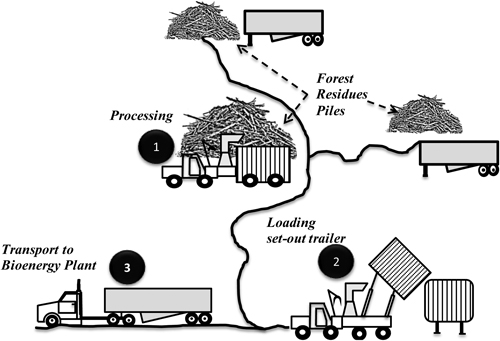
Fig. 1. Mobile chipper processing different piles of forest residues and loading the chips into trailers. The number located in the black circles describes the phases of the process.
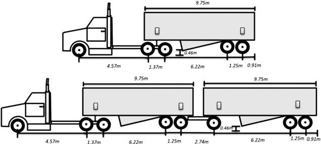
Fig. 2. Two typical tractor-trailer configurations, a) 6x4 tri-axle truck and single trailer approximately 15.5 t of capacity; b) 6x4 tri- axle truck and double trailer (9.75 and 9.75 m in length), with a capacity of 27.3 t.
We used the continuous time study method (Pfeiffer 1967), to determine the time consumed chipping and transporting the residues. This study was also complemented by the guidelines provided in Bjorheden and Thompson. (1995). We combined manually timing, video recording and spatial-temporal tracking analysis of machine and truck movements to accurately collect the data. One hundred and twenty cycle times for chipping and twenty round-trips for transportation were recorded. A cycle time consist of processing and dumping into the trailer one chipper container load.
Four chipping elements were identified and timed to determine the total delay free cycle time: (i) chipping includes the conversion of forest residues into chips; (ii) traveling begins at the end of the chipping process when the chipper bin is full with chips and moving to the trailer to dump the load and ends before the dumping process is performed; (iii) dumping begins at the end of traveling and ends when the load has been dumped in the trailer; (iv) returning begins at the end of the dumping process and ends when the machine is back to the pile before the start of a new chipping process. The amount of chips processed in each cycle was also recorded from the internal weight scale of the mobile chipper. In addition to the total cycle time, delay times were considered. Scheduled and un-scheduled downtimes for chipping were also recorded.
For the transportation systems the following variables were recorded: (i) unloaded travel time, is the time spent by the truck travelling between the plant and the forest when the truck is unloaded; (ii) loaded travel time, is the time spent by the truck traveling between the forest and the plant when the truck is loaded; (iii) dumping time spent by the truck while is being unloaded at the plant; (iv) truck turning around; and (v) hook and unhook time in the forest is the time spent by the truck while the empty trailer (or trailers when running double trailers) is unhooked and the loaded trailer is hooked in the forest. Non-scheduled downtime in transportation was considered although none occurred during the study period.
GPS receivers Visiontac® were placed in the chipper and trucks in order to collect spatial and temporal information of their movements. The GPS devices recorded the position and time at a rate of one coordinate per second. In a normal shift of 10 hours, we recorded an average of 28 800 points. No significant problems with satellite reception related to tree canopy interference were found since all the study areas were cleared (clear-cut harvesting) before the biomass recovery operation was carried-out.
Collected data from the GPS devices was pre-processed using a digital toolbox based on an algorithm developed in Python programming language for ArcGIS 10 software (ESRI 2012). In the preprocessing procedure we filtered the data to reduce the amount of identical coordinates and produce a spatial-temporal layer suitable for tracking analysis. Tracking analysis, an extension from ArcGIS 10, was used to recreate the movement patterns of the chipper and trucks. We also calculated travel distances from the spatial data.
Average cycle time for the chipper per activity for the four units analyzed is shown on Table 1. On average, about 76% of the time (delay free) the machine was chipping or waiting for the next piece to be fed. About 18% of the time the chipper was moving to the dumping site and travelling back to the forest residues pile. The rest of the time was spent in dumping. The range of values for chipping time is wide, 8.07 to 40.78 minutes (Table 1). Since this range is based on the average values of all units, it was considered an indicator of the high sensitivity of this process to the type of material and site characteristics. Average productivity for the four units was estimated as 12 green tonnes per productive machine hour.
| Table 1. Statistics of time spent in each activity of the productive chipping cycle. | |||||
| Mean | Min | Max | SD | % | |
| Chipping (min) | 16.45 | 8.07 | 40.78 | 5.52 | 75.80 |
| Travelling to trailer (min) | 1.83 | 0.47 | 6.73 | 1.12 | 8.44 |
| Dumping (min) | 1.46 | 0.45 | 3.07 | 0.51 | 6.74 |
| Returning to pile (min) | 1.96 | 0.25 | 6.62 | 1.30 | 9.02 |
| Total (min) | 21.70 | 9.24 | 57.20 | 8.46 | 100.00 |
| Bin-load (Green tonnes) | 4.09 | 2.09 | 6.01 | 0.70 | |
2.2 Distribution fitting and parameter estimation
Distributions were fitted for each activity in the chipping productive cycle (Table 2). The Input Analyzer from Rockwell Arena Simulation Software (Rockwell Automation 2012) was used to estimate the distribution and parameters that fit best to each dataset. We evaluated the p-values of the chi-squared goodness of fit test and squared errors to determine if enough evidence has been provided to say that the data is well represented by the suggested distribution. We fitted distributions to time spent (minutes) in the chipping and dumping process. Chipper travelling time was modeled as a function of the distance between the trailer and the pile. We calculated the chipper speed variability while the machine was travelling. Diagnosis was performed for all distributions using quantile-quantile (Q-Q) and probability-probability (P-P) plots and the results were approximately linear for all the selected distributions.
| Table 2. Fitted distributions for each operational process. | |||||
| Process | Probability distribution | Location parameter | Scale parameter | Shape parameter | Squared error and p-values |
| Chipping sorted (min) | Erlang | 8 | 1.63 | 4 | 0.0056; p > 0.75 |
| Chipping unsorted (min) | Gamma | 11 | 5.91 | 1.53 | 0.0023; p = 0.31 |
| Travelling to trailer (m/min) | Weibull | 1 | 44.3 | 1.66 | 0.0048; p = 0.51 |
| Dumping (min) | Log-Normal | 0.18 | 1.28 | 0.527 | 0.0042; p = 0.38 |
| Returning to pile (m/min) | Gamma | 6 | 14.7 | 2.16 | 0.0011; p = 0.73 |
| Bin-load (kg) | Normal | 4090 | 692 | 0 | 0.0116; p = 0.05 |
For the transportation part of the model, the unloading time (normal distribution μ = 59.4, σ = 15, in minutes), hook and unhooking time (Erlang λ = 1.91, k = 1, a = 2, in minutes), were considered stochastic components. Truck loaded and unloaded travel time was modeled deterministically using the relation between the average driving speed and the distance since no significant sources of uncertainty were identified in this stage of the process.
2.3 Discrete-event simulation model
The discrete-event simulation model was designed in the Rockwell Arena Software environment. A two component model was developed. The first component expresses the different stages involved in the mobile chipping productive cycle. The second component simulates trucks arriving to the processing site and transporting the material to the bioenergy facility. Both components start with the creation of entities. Entities are usually material objects that flow through the system and produce a change in the output or state of the system (Kelton et al. 2001). The mobile chipper represents an entity for the chipper model. Trucks arriving to the system are the entities of the transportation model. Entities are recycled in the model until the scheduled time is reached.
Inputs for the chipping model are the scheduled machine hours in a day including scheduled downtimes, and the average distance between the trailers and the piles. Also the average time spent moving between piles can be added in the model. This value can be calculated by the analyst by counting the number of piles, measuring the average distance between them and relating this value to the average speed of the chipper (5 km/h).
The trucking model assumes that the planner has the complete control of the number of trucks, trailers, and truck arrival schedule. The transportation model’s inputs are the average speed of the truck on highway paved roads (from the bioenergy facility to the entrance of the unit), and within the harvest unit driving on the forest roads (gravel or dirt roads), the distance between the entrance of the unit and the processing site, and the average distance between the residue piles and the turn-around.
For the mobile chipper model, the first stage in the model occurs when the chipper proceeds to process the residue in a pile. (Fig. 3a). The next stage involves a decision module that is linked with the transportation model. If an empty trailer is available to dump the load, then the chipper continues to the next stage which is travelling to the trailer, and then unloading the processed material. If a trailer is not available then thge chipper travels to the landing (where the trailer will be placed) and then waits until an empty trailer is available. The trailer is modeled as a tank with a fixed capacity depending on the size of the trailer. Once the unloading process is finished the chipper begins to travel to the pile. This stage captures the variability of the chipper driving at different speeds.
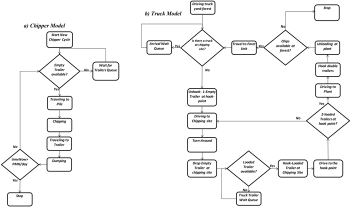
Fig. 3. Model logic: a) chipper; b) truck-double trailers. View larger in new window/tab.
The amount of processed chips (metric tonnes) in each productive cycle has a partial positive correlation with the chipping time and was estimated using the procedure proposed by Mykytka and Cheng (1994) to generate correlated random variables obtained from independent distributions. The mathematical expression to calculate the bin load size Y2 as a function of the chipping time X, given the Pearson correlation coefficient ρ is expressed as follows:

where
Y2 = correlated random variable of the amount of chips produced in each cycle time (kg)
Y = uncorrelated random variable of the amount of chips produced in each cycle time (kg)
X = random variable representing the chipping time (min)
μx = mean of the chipping time distribution (min)
μy = mean produced chips per cycle distribution (kg)
σx = standard deviation of chipping time distribution (min)
σy = standard deviation of chips produced per cycle distribution (kg)
ρ = Pearson correlation coefficient between chipping time and chips produced per cycle
Chipper downtime was divided into two categories: the scheduled downtime, which has to be made on a daily-basis to change the knives, warm the engine and clean the filters, and the unscheduled downtime that is caused by unplanned mechanical problems. One of the most common causes of mechanical downtime is related to the presence of metal cables or debris inside the pile. We modeled unscheduled delay using a Poisson distribution with parameter λ = 550, which represents the number of processed chipper bins before a downtime occurred. This parameter was estimated using the average of incidence of this problem in the last 6 months. Other non-mechanical related unscheduled downtimes such as planning breaks and supervisor visits were not considered in this study however if the analyst has data related to the frequency and duration of these delays they can be added to the model.
The logic for the transportation model (Fig. 3b) begins when an empty truck leaves the truck yard to go to the forest unit. The truck then drives to the processing site, turns around and places the empty trailer. The next step is to drive to a loaded trailer, hook it and travel back to the mill. In the double trailer setting, due to road accessibility, the truck must drop one of the empty trailers before continuing to the pile location. The mobilization within the unit is modeled as a function of the internal distances and the speed of the truck. The first truck arrives one hour after the chipper starts the chipping process (it is assumed that reserve empty trailers are left in the unit the day before the operation starts, the second truck arrives 30 minutes after the first truck has arrived. The model assumes single passage forest roads which limits one truck to enter into the system at each time. If double trailers are used the truck must pick up each trailer one at a time. This factor increase the cycle time considerably compared to single trailer configuration. An increase in round-trip time of around 30% is expected when using double trailers (for a roundtrip-distance of 120 km on paved roads and 5 km in gravel roads). The time to setting up double trailers increases as the distance between the hook-up point and processing site increases. Also the dumping time at the bioenergy facility increases for double trailers.
2.4 Costing model
Costs were estimated using information from the different stakeholders in the forest biomass supply chain. This includes consultation with contractors, trucking companies, forest managers, landowners and bioenergy facilities. Costs were calculated for the mobile chipper and trucks described in section 2. The cost model accounts for standing times due to truck-machine interactions.
Processing and transportation costs were separated into two main categories: fixed and variable costs. We first calculated the hourly variable and fixed cost in order to be able to model the cost in each activity based on the time spent. Operational and standing costs were then calculated for the chipper and trucks.
Fixed cost of mobile chipping and transportation was based on salvage value, annual depreciation, average yearly investment, interest, insurance and taxes. We assumed 2000 scheduled machine hours per year for the chipper based on historical machine records. For transportation, we assumed 2200 scheduled machine hours per year.
Variable costs for chipping comprised labor, fuel, repair and maintenance. Additionally to fixed and variable costs, operational costs for chipping include overhead and profit and risk costs. Overhead cost ($19.67/h) included supervision (assuming that general supervisors spend 10% of the total working time in chipping operations), communications (radio and cell phones) and administration cost (secretary and office consumables). Supportive equipment includes one water truck ($7.33/h), service truck ($9.47/h) and operator’s pickup truck ($11.37/h). These costs are incurred whether the chipper is operating or standing. Profit and Risk was estimated as 7% of the sum of fixed, variable, supportive equipment and overhead costs. Chipping operational costs were calculated based on Eq. 2.
![]()
where
OCch = hourly processing cost while the machine is operating ($/h)
Fxch = fixed costs for chipping ($/h)
Vach = variable costs for chipping ($/h)
Rpch = risk and profit for chipping ($/h)
Such = supportive equipment hourly cost for chipping ($/h)
Ovch = overhead hourly cost for chipping ($/h)
Chipper standing costs were calculated as the sum of an opportunity cost based on the expected profit the chipper would have earned if it had been operating, plus labor, interest, insurance, supporting equipment and overhead (Eq. 3). Since the machine is assumed to be idle during waiting, no depreciation cost was included, given that the machine is not being used. Obsolescence is not considered in this study, since we assumed that the useful life of forest machinery is dependent on the hours worked, not the passage of time as it occurs in the software industry or electronics for example.
![]()
where
ICch = hourly chipper standing cost ($/h)
Intch = hourly interest cost for chipping ($/h)
Insch = hourly insurance and taxes cost for chipping ($/h)
Lach = hourly insurance and taxes cost for chipping ($/h)
For Transportation, variable cost includes labor, repair and maintenance, fuel and lubricants. Variable cost is a function of distance, road surface (gravel, paved dirt), speed and weight of the truck and trailer (loaded or unloaded). Only one driver is required per truck. Fuel cost was estimated as a function of the truck power necessary to overcome rolling and air resistance forces. Rolling and air resistance are dependent upon the speed, weight (empty or loaded) and roundtrip distance. Variable transportation costs for transportation were calculated in the following section for the validation unit, based on the traveled distance, and weight (loaded unloaded), on different road surfaces.
Transport operational cost (Eq. 4) includes 7% percent of risk and profit of variable fixed and overhead costs. Overhead transportation cost was calculated based on dispatching, communications and administration costs. Transportation standing costs were calculated following Eq. 5.
![]()
![]()
where
Fxt = truck hourly fixed costs ($/h)
Varwz = truck hourly variable costs ($/h)
Rpt = truck hourly risk and profit ($/h)
OCTrwz = operating truck hourly processing cost on road surface r with a load w and speed z ($/h)
OCt = truck hourly standing cost ($/h)
Intt= truck hourly interest cost ($/h)
Inst = truck hourly insurance and taxes cost ($/h)
Lat = truck hourly labor cost ($/h)
Ovt = truck overhead hourly cost ($/h)
Total chipping (Eq. 6) and transportation (Eq. 7) cost per tonne of chips ($/t) were calculated taking into account the time spent in each activity listed in the simulation model. A final cost equation includes previous costs, the mobilization cost of the machinery to the forest unit using a highway legal lowboy, mobilization cost to drop the extra trailers at the site and stumpage price of the piled material if any (Eq. 8).


where
TCch total chipping cost as a function of the amount of processed chips ($/green t)
tc = time spent chipping (h)
tp = time spent moving to pile (h)
tm = time spent moving to trailer (h)
td = time spent dumping in trailer (h)
tw = chipper standing time (h)
tb = standing time due to unscheduled machine breakdowns (h)
tl = standing time due to scheduled machine downtimes (h)
Q = amount of chips processed (t)
TCt = total transportation costs ($/green t)
trwz = truck time spent traveling on road surface r with a load w at a speed z (h)
tx = truck standing time waiting for loaded containers (h)
ty = truck standing time due to truck queue in the forest (h)
th = time spent to hook a single or double containers (h)
ti = unloading time at the bioenergy facility (h)
Mvu = mobilization cost of the machinery to the unit ($)
Stp = stumpage cost ($/green t)
mc% = moisture content green basis (%)
COST = total cost per tonne ($/dry matter t)
Assumptions and supportive equations for fixed and variable chipping and transportation cost calculations are available as a supplementary file.
2.5 Validation study area
We made an independent validation of the model (additional to the previous four evaluated units) to estimate the degree of accuracy of the model to represent the chipper and truck productivity. The validation was performed in a forest unit with an area of 16.2 ha located in the Coast Range in western Oregon, United States 123°28´W, 43°28´N. The access to the unit was characterized by steep loose-gravel roads with road gradients ranging from 8 to 20%. The area was harvested in late April 2012 using cable-logging equipment. Piles of forest residues were left in the forest around the landings as a by-product from the logging operation. The residue piles were composed of a mixture Pseudotsuga menziesii (Douglas-fir), Abies concolor (white-fir) and Libocedrus decurrens (incense-cedar) with pieces ranging from 10 to 20 cm in diameter and 0.9 to 3 m in length. The distance from the main road entrance to the processing site was 2.57 km. Average distance between the trailer locations and the piles was 40 m. Fifteen piles were distributed within the unit with an average distance between piles of 70.6 m. Turn-around average distance to the piles was 150 m. Double trailers as shown on Fig. 2b, were used in the transportation of chips. Two trucks transported the chips to the plant. The distance between the forest unit entrance (hook-up point) and the plant was 50 km.
Thirty independent repetitions were made to evaluate the performance of the model; the average was compared to the actual value. Welch’s t-test was used to assess if there was statistical significant difference between modeled and actual data. Given the multiple outputs of the simulation model (chipping time, traveling to trailer, chips produced, etc.), the Bonferroni inequality was used to calculate the critical t-value for multiple responses. The critical value using this approach is tm–1;α/2T, where m is the degrees of freedom (30-1), T is the number of responses (5) and α is the significance. We combined the Bonferroni inequality with a significance value of α = 0.20, suggested by Kleijnen (1995) for simulation models with multiple responses.
2.6 Optimization scenarios
We developed different scenarios using the simulation model to analyze the effect of the main variables on productivity and strategies to reduce the cost and increment the marginal net profit under uncertainty. We focused our analysis on the effect of truck-chipper interactions on productivity. In all scenarios we modeled productivity and cost for a 10-hour mobile chipper shift. Other assumptions include: (i) all forest roads were single passage; (ii) only two reserve trailers were available for the chipper; (iii) the average distance from the trailer to the pile was 40 m; (iv) the average distance from pile to turn-around was 150 m; (v) The hook-point for double trailers was located in the entrance of the unit; and (vi) the moisture content was 30% (wet basis).
Available transportation options were: (a) two single trailer trucks, (b) three single trailer trucks, (c) two double trailer trucks and (d) three double trailer trucks. Longer trailers (>9.75 m) are available but forest road conditions constraint their access. Other double trailer configurations are available (i.e. 6.1–12.2 m in length) but the option 9.75–9.75 m maximizes the maximum allowable weight (47 854 kg) and the tractor-trailers length (24.38 m), under the current road regulations.
In the first scenario we modeled the chipper and truck productivity as a function of the distance between the entrance forest unit and the bioenergy facility (highway distance). We ran three simulations for roundtrip highway distances ranging between 40 km and 280 km. We assumed a fixed round-trip distance in forest roads of 6 km from the entrance of the unit to the pile location.
In the second scenario we estimated productivity and cost as a function of the forest road distance from the entrance of the unit (trailer hook-up point) to the residue pile location. In this scenario we set the round-trip distance to the bioenergy plant equal to 120 km, and changed the round-trip internal distance from 2 to 12 km. All other inputs remained the same as in scenario 1.
The third scenario estimates the effect of reducing chipper moving time (traveling to pile and trailer) on productivity and cost. Trailer-to-pile distance was set to zero. We modeled the estimated productivity dumping directly into the trailer or blowing into the trailer using an extension accessory on the chip tube. We assumed bulk density of the dumped and blown chips in the trailer would be the same.
3 Results
3.1 Model Validation
For the validation study area we compared the results of the simulation against the actual data obtained from a time and motion study (Table 3). We calculated the critical value t29;0.02 = 2.46 for the validation data of the model. No statistical difference was found between the model and the actual data for each of the components of the chipper cycle time and the amount of chips produced. All their respective t values were below the critical value of 2.46.
| Table 3. Modeled and actual results for the validation study. | |||
| Process | Actual | Model | % difference |
| Chipping (min) | 882.99 | 893.59 ± 18.00 | 1.20, t29 = 1.492 |
| Travelling to trailer (min) | 101.52 | 107.75 ± 8.84 | 6.14, t29 = 1.734 |
| Dumping & record keeping (min) | 89.28 | 89.53 ± 3.50 | 0.28, t29 = 0.174 |
| Returning to pile (min) | 91.10 | 88.24 ± 4.14 | 3.14, t29 = 1.700 |
| Chips produced (t) | 277.72 | 279.36 ± 7.57 | 0.59, t29 = 2.329 |
| Total productive time (min) | 1164.88 | 1153.53 | 1.22 |
| Productivity (Green tonnes/productive hour) | 14.30 | 14.22 | 0.62 |
3.2 Economics of mobile chipping under uncertainty
The economics of mobile chipping is a function of the chipper productive time, transportation time and machine interactions that may cause delays in processing or transporting. Specifically, costs in mobile chipping are affected by chipper and truck standing times, distance between the forest unit and the plant, internal road distances and conditions (i.e. gravel and single passage road), pile location, physical properties and characteristics (size) of the forest residues. To illustrate the effect of these variables on productivity we calculated the cost for the forest area used in the validation using the cost model.
Chipping costs were separated for each of the activities in the productive cycle of the chipper. We considered chipping, moving to trailer, moving to pile and dumping as operational stages, therefore the operational cost is calculated by multiplying the operating cost by the accumulated time spent in the unit (Table 4).
| Table 4. Estimated hourly cost for the Bruks chipper under the study conditions. | ||
| Cost $/hour | Operating | Standing |
| Interest, insurance, and taxes | 116.75 | 36.75 |
| Labor | 37.50 | 37.50 |
| Knife cost | 16.00 | - |
| Repair and maintenance | 56.00 | - |
| Fuel cost | 48.00 | - |
| Oil and lubricants | 17.64 | - |
| Total variable cost | 175.14 | 37.50 |
| Supportive equipment | 28.18 | 28.18 |
| Overhead | 19.67 | 19.67 |
| Profit and risk (7%) | 23.78 | 23.78 |
| Total $/hour | 363.51 | 145.87 |
Operational transportation cost was calculated as a function of the time spent: (i) arriving to the site; (ii) driving in forest roads empty and loaded; and (iii) turning-around. Standing transportation costs were calculated based on: (i) hook and unhook time; (ii) unloading at the plant and (iii) standing time due to chipper-truck interactions (Table 5).
| Table 5. Hourly transportation costs based on road standard and if truck is traveling empty or loaded. Single trailer is 9.8 m and double trailer is composed of two 9.8 m trailers. | ||||
| Truck-trailer configuration ($/h) | Paved | Gravel | Dirt | Standing |
| Single trailer truck empty | 80.32 | 68.37 | 65.73 | 45.34 |
| Single trailer truck loaded | 96.06 | 76.72 | 73.44 | 45.34 |
| Double trailer truck empty | 98.53 | 78.97 | 75.03 | 50.87 |
| Double trailer truck loaded | 126.19 | 92.11 | 89.03 | 50.87 |
Maximum allowable tractor-trailer weight (Table 6) was calculated using a linear programming model proposed by Sessions and Balcom (1989), that it is based on axle-load group limits for the single and double trailer options. Double trailers required an additional axle (dolly) to connect both trailers. This axle adds weight and cost to this configuration.
| Table 6. Truck and trailer specifications. | ||
| Truck specifications | Single trailer truck (15.5 t) | Double trailer truck (27.3 t) |
| Truck weight (t) | 9.1 | 9.1 |
| Trailer weight (t) | 3.9 | 10.2 |
| Maximum capacity (t) | 15.5 | 27.3 |
| Number of axles | 5 | 9 |
In economic terms, the hourly cost of double trailers is 30% more than a single trailer configuration but the maximum allowable load increases by 76%. However, the use of double trailers requires the additional time to hook and unhook the trailer combination and a suitable location to do so. Transportation cost per hour decreases on gravel and dirt roads because it is assumed that at low speeds in gravel (15 km/h) and dirt (5 km/h) roads fuel consumption per hour decreases even though rolling resistance increases. We assumed an average speed in paved roads of 70 km/h.
Hourly cost was then related to the total amount of chips produced in order to calculate the cost per tonne. We incorporated the moisture content of the chips to obtain the rate per dry tonne of chips since the product was used in power generation. Moisture content was estimated as 30% (wet basis) from 36 samples. Estimated costs per dry matter tonne (DMt) were $37.94/DMt for chipping, $3.60/DMt for machinery mobilization and placement of reserve trailers at the chipping site (assuming six hours of a highway lowboy with an hourly cost of $100 and 2 hours of truck waiting time), and $18.13/DMt for transportation giving a total of $59.66/DMt (Fig. 4).
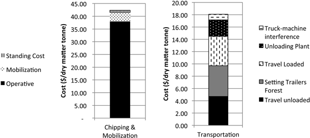
Fig. 4. Total cost of chipping and transportation for the validation forest unit.
Using the simulated data we created a probability histogram for the total cost per dry matter tonne given the variability of the system (Fig. 5). This histogram can help risk adverse managers to analyze the probability of occurrence of each cost for a particular unit and evaluate if it is profitable or not to do an operation. In this case, there is a 76% probability to have a cost between $55 and $61/DMt and 24% probability to have a cost between $61/DMt and $69/DMt.
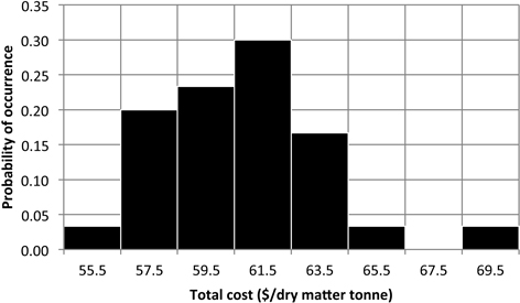
Fig. 5. Probability of total chipping and transportation cost for the validation forest unit.
3.3 Optimization of mobile chipping and truck-chipper interactions
3.3.1 First scenario
Results showed that for transportation options (a), and (c) chipping cost ($/DMt) increases as distance increases (Fig. 6). This trend is caused by the increasing standing time of the chipper (Fig. 7). As distance increases the truck has to spend more time traveling loaded and unloaded to the plant and back to the unit and therefore it is difficult to reach the forest site in time to replace the loaded trailers. The cost impact is higher when using only two single trailer trucks because the amount of transported chips per trip is less than the double trailer configuration. Using three double trailer trucks or three single trailer trucks has the minimum impact on the chipping cost per tonne because the standing time of the chipper is minimized, however transportation cost increases. Transportation cost is mainly affected by the increase in round-trip distance and number of trucks. As the number of trucks increases there is a high probability of truck congestion in the single passage roads. Each truck has to wait for other trucks and loaded trailers. Transportation cost in options (a) and (b) are mainly affected by the maximum allowable weight for singles. Due to their reduced capacity, the number of trips is higher compared to the double trailer truck configuration. Options (c) and (d) are lower cost because the double trailer configuration can carry more per trip (Fig. 8). Options (b) and (d) are more affected by truck standing times. The additional truck under this configuration adds more congestion at the arrival to the unit (Fig. 9). Although adding a truck can minimize the standing time of the chipper, the additional truck may not be able to complete the number of trips necessary to satisfy a normal working shift for the trucks (8-hours). The under-utilized truck cost was calculated by multiplying the hourly standing cost of the truck and the hours necessary to complete a minimum working shift of 8 h. Focusing only on the chipping cost, the manager may choose option (d), 3 doubles, as the most cost effective for the operation since that is the one that maximizes chipper utilization rate and appears to be less sensitive to the distance. However, transportation cost indicates that the less expensive option is (c), 2 doubles.
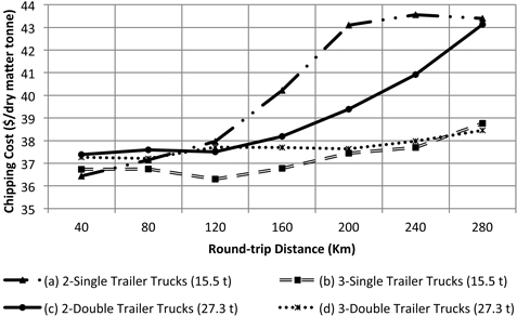
Fig. 6. Chipping cost as a function of the round-trip highway distance to bioenergy plant. Internal forest round-trip distance was fixed at 6 km.
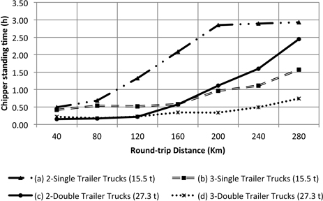
Fig. 7. Chipper standing time as a function of round-trip highway distance to bioenergy facility. Internal forest round-trip distance was fixed at 6 km.
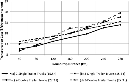
Fig. 8. Transportation cost as a function as a function for round-trip highway distance to the bioenergy facility. Internal forest round-trip distance was fixed at 6 km.
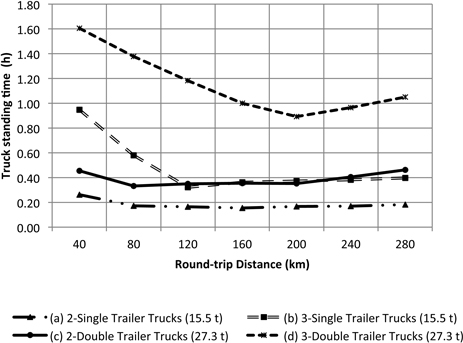
Fig. 9. Truck standing time at arrival due to road congestion and waiting for loaded trailers. Internal forest round-trip distance was fixed at 6 km.
Adding chipping and transportation cost to account for truck-chipper interactions (Fig. 10) we determined that the use of two double trailer trucks is the most cost-effective option for round-trip distances of less than 220 km. For round-trip distances greater than 220 km the use of three double trailer trucks seems to be more effective. For round-trip distances around 40 km options (a) and (c) appear to have the similar costs.
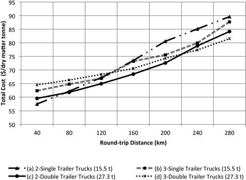
Fig. 10. Total costs as a function of the round-trip highway distance to the bioenergy plant. Internal forest round-trip distance was fixed at 6 km.
3.3.2 Second scenario
Total costs of processing and transport were significantly more sensitive to the in-forest road distance than to the highway road distance (Fig. 11). For the two double trailer trucks configuration, a change in the forest road distance from one to six kilometers caused an increase of 18% in the total cost. This change is caused by the low travel speed on forest roads (steep roads and tight curves) and the time the truck spends turning-around, hooking and unhooking trailers.
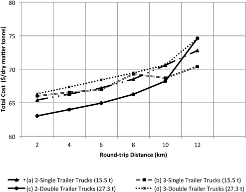
Fig. 11. Total costs as a function forest road distance for a highway haul round-trip distance of 120 km to the bioenergy plant.
Productivity of double trailer trucks is more sensitive than single trailer trucks to increases of internal road distance, due to significant increases in round-trip travel time (steeper curves on Fig. 11). However, the use of two double trucks appears to be the most cost effective configuration because fewer trips to the plant are required compared to single trailer configurations for round-trip in-forest distance of less than 10 km. For in-forest distances greater than 10 km the use of three single trucks is cheaper that the all the other options because chipper utilization is increased compared to the other alternatives.
3.3.3 Third scenario
The mobile chipper spends around 17% of the productive cycle, moving between the trailer and the pile. Reducing the moving time may increase the productivity by allowing the chipper to spend more time chipping or feeding the machine. Cost and productivity were modeled under these considerations for Scenario 3. Results show that eliminating the moving time but dumping into the trailer decreases the overall cost about 7% (Fig. 12). Blowing the material directly into the trailers reduces the cost about 8% and this option becomes limited by the availability of trailers. Adding one more double trailer truck minimizes the chipper standing time and decreases the overall cost by 22% with respect to the actual value (Fig. 12, D). Any machinery or trucks necessary to transport the material to a centralized landing must cost $5.40 to $15.92/DMt or less to be a feasible option as compared to the base scenario. Additionally a centralized landing may require clearing a large area to allow for the placement of trailers and residues and to allow the trucks to turn-around.
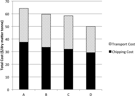
Fig. 12. Total costs for chipping at centralized landing with no machine movement. A) Actual cost using two double trailer trucks; B) total cost operating with no chipper movement and direct dumping into trailers and using 2 double trailer trucks; C) total cost with no machine movement but blowing directly the material into trailers and using two double trailer trucks; D) total cost with no machine movement but blowing directly the material into trailers and using three double trailer trucks.
4 Discussion and conclusions
We presented a stochastic simulation model and optimization procedure applied to forest biomass recovery operations for energy purposes. The proposed stochastic simulation model has been shown to be an accurate tool to support decisions related to the estimation of productivity under uncertainty. The forest biomass processing and transportation was modeled as a dynamic system, providing productivity estimates of each activity in the productive cycle accounting for truck-machine interactions.
On steep terrain conditions it is important to consider the impact of road characteristics that can affect truck-machine interactions. Important road characteristics to considering when planning operations on steep slopes are internal forest distance, type of road surface, road width, road grade and curve radii that can limit the access to high capacity trucks due to off-tracking.
Standing times for the chipper and trucks due to truck-chipper interactions must be considered and quantified when analyzing economics and productivity of the forest biomass collection. A costing method was developed to account for the cost while the chipper or trucks are operating or standing. Assigning value to the standing cost of the chipper and trucks allowed us to optimize the operation by minimizing chipper and trucks standing costs. Reducing the chipper standing time may require additional trucks but as number of trucks increases the probability of truck congestion at arrival to the forest unit increases. Additionally some trucks cannot be fully utilized incurring in higher transportation cost. In this study trucks had to be paid for a minimum day. In other situations, truck dispatching to other jobs may improve truck efficiency.
Single passage road distances may limit the number of trucks that can reach the processing site at each time, thus affecting costs and productivity of the chipper and trucks. Total cost is highly sensitive to small increases in distance especially for double trailer configurations that require several internal trips to drop off, collect, and assemble the double trailer configuration.
For the study site the use of two double trailers is the most cost-effective option on steep terrain. The capacity of this configuration compensates the additional time spent in the forest. This configuration was selected by comparing its productivity and cost with alternative transportation systems and number of trucks.
The model was able to estimate a cost distribution that can be used to assess the risk of operating in some forest units. In cases where delivery prices were close to expected cost estimations a deep analysis of the distribution can improve decision making process and analyze the potential trade-offs of operating in some units.
The proposed simulation model attempts to explain complexity of a real mobile chipping system by simplifying it into discrete parts. Simplification can lead to some sources of error and the analyst has to be aware of them. The model simulates chipping operations as if the residues were located in one single location. In reality, residues are distributed among different piles and locations. Also we have a fixed capacity of trailers (13 650 kg for each trailer in a doubles configuration and 15 500 kg for singles), but in reality the maximum amount of chips dumped in each trailer varies. This causes some amount of chips to remain in the reserve trailers after a working shift without being transported. To minimize this problem we assumed that those chips will remain in the reserve trailers and eventually will be transported the next day when the trailers are full. We input the average of the distance to the turn-around and between the trailer and the pile, but in a harvest unit where the standard deviation is high, using the average value may lead to inaccurate results. Also, the model does not consider that productivity and knife sharpness are correlated; i.e. productivity should be highest after a knife change and become lower as more chips are processed (Nati et al. 2010). Additionally the model does not consider the loss in productivity due to operator fatigue. Finally the model is intended to support the decision making process but not remove the final decision from the analyst.
Future work could evaluate establishing a centralized yard to reduce chipper standing time, reduce chipper moving time and increase large trailer access. However, benefits must also consider the additional costs of aggregating the material.
Finally, combining the use of GPS, geographical information systems, spatial-temporal analysis and discrete-event simulation proved to be effective in constructing a robust model to estimate the economics of mobile chipping. These methods can be applied to analyze other forest operations.
References
Asikainen A. (2010). Simulation of stump crushing and truck transport of chips. Scandinavian Journal of Forest Research 25: 245–250. http://dx.doi.org/10.1080/02827581.2010.488656.
Baumgras J., Hassler C., LeDoux C. (1993). Estimating and validating harvesting system production through computer simulation. Forest Products Journal 43(11/12): 65–71.
Biomass Energy Resource Center (2007). Woodchip fuel specifications and procurement strategies for the Black Hills. South Dakota Department of Agriculture Resource, Conservation and Forestry Division. 31p. http://www.sdda.sd.gov/Forestry/Publications/PDF/Black%20Hills%20Wood%20Fuel20Specifications%205.15.07%20FINAL%20.pdf. [Cited 23 February 2012].
Bjorheden R., Thompson M.A. (1995). An international nomenclature for forest work study. Proceedings IUFRO 1995, XX World Congress. IUFRO. p. 190–215.
Bracemort K. (2012). Biomass: comparisons of definitions in legislation through the 112th Congress. CRS Report R40529. Congressional Research Service, Washington DC. 17 p.
Bradley P., Biltonen F., Winsauer S. (1975). A computer simulation of full-tree field chipping and trucking. U.S. Department of Agriculture, Forest Service, North Central Forest Experiment Station, Research Paper NC-129. 14 p.
BRUKS (2010). Mobile chippers. http://www.bruks.com/en/products/Mobilechippers/8052/8052-STC/. [Cited 23 February 2012].
ESRI (2012). ArcGIS 10. http://www.esri.com/software/arcgis/arcgis10. [Cited 3 October 2012].
Gallis C. (1996). Activity oriented stochastic computer simulation of forest biomass logistics in Greece. Biomass and Bioenergy 10(5): 377–382. http://dx.doi.org/10.1016/0961-9534(96)00002-5.
Hakkila P. (1989). Utilization of residual forest biomass. Springer-Verlag, Berlin. 568 p. http://dx.doi.org/10.1007/978-3-642-74072-5.
Kelton D., Sadowski R., Sadowski D. (2001). Simulation with Arena. Second edition. McGraw-Hill, Boston. 611 p.
Kleijnen J. (1995). Verification and validation of simulation models. European Journal of Operational Research 82(1995): 145–162. http://dx.doi.org/10.1016/0377-2217(94)00016-6.
McDonagh K., Meller R., Visser R., McDonald T. (2004). Harvesting system simulation using a systems dynamic model. Southern Journal of Applied Forestry 28(2): 91–99.
Mikytka E., Cheng C. (1994). Generating correlated random variates based on an analogy between correlation and force. Proceedings of the 1994 Winter Simulation Conference. p. 1413–1416.
Mobini M., Sowlati T., Sokhansanj S. (2011). Forest biomass logistics for a power plant using a discrete-event simulation approach. Applied Energy 88(4): 1241–1250. http://dx.doi.org/10.1016/j.apenergy.2010.10.016.
Northwest Advanced Renewables Alliance (2011). http://www.nararenewables.org/. [Cited 16 February 2012].
Nati C, Spinelli R., & Fabbri P. (2010). Wood chips size distribution in relation to blade wear and screen use. Biomass and Bioenergy 34: 583–587. http://dx.doi.org/10.1016/j.biombioe.2010.01.005.
Pfeiffer K. (1967). Analysis of methods of studying operational efficiency in forestry. Master of Forestry Thesis. University of British Columbia. 94 p.
Rockwell Automation (2012). Arena simulation software. http://www.arenasimulation.com/Arena_Home.aspx. [Cited 16 February 2012].
Sessions J., Balcom J. (1989). Determining maximum allowable weights for highway vehicles. Forest Products Journal 39(2): 49–52.
Smith B., Miles P., Perry C., Pugh S. (2009). Forest resources of the United States, 2007. U.S. Department of Agriculture, Forest Service, Washington Office, General Technical Report WO-78. 336 p.
Spinelli R., Hartsough B. (2001). A survey of Italian chipping operations. Biomass and Bioenergy 21: 433–444. http://dx.doi.org/10.1016/S0961-9534(01)00050-2.
Spinelli R., Visser R. (2009). Analyzing and estimating delays in wood chipping operations. Biomass and Bioenergy 33: 429–433. http://dx.doi.org/10.1016/j.biombioe.2008.08.003.
Talbot B., Suadicani K. (2005). Analysis of two simulated in-field chipping and extraction systems in spruce thinnings. Biosystems Engineering 91(3): 283–292. http://dx.doi.org/10.1016/j.biosystemseng.2005.04.014.
Staudhammer C., Hermansen-Baez L., Carter D., Macie E. (eds.). (2011). Wood to energy. Using southern interface fuels for energy. U.S. Department of Agriculture, Forest Service, Southern Research Station, General Technical Report GTR-132. 90 p. http://www.interfacesouth.org/products/publications/wood-to-energy-using-southern-interface-fuels-for-bioenergy/index_html. [Cited 23 February 2012].
Taguchi G. (1987). System of experimental designs. Vols. 1 and 2. UNIPUB/Krauss International Publications, New York.
Total of 28 references
Send to email
