Sakari Tuominen  ,
Juho Pitkänen,
Andras Balazs,
Kari T. Korhonen,
Pekka Hyvönen,
Eero Muinonen
,
Juho Pitkänen,
Andras Balazs,
Kari T. Korhonen,
Pekka Hyvönen,
Eero Muinonen
NFI plots as complementary reference data in forest inventory based on airborne laser scanning and aerial photography in Finland
Tuominen S., Pitkänen J., Balazs A., Korhonen K. T., Hyvönen P., Muinonen E. (2014). NFI plots as complementary reference data in forest inventory based on airborne laser scanning and aerial photography in Finland. Silva Fennica vol. 48 no. 2 article id 983. https://doi.org/10.14214/sf.983
Highlights
- Using NFI plots in forest management inventories could provide a way for rationalising forest inventory data acquisition
- NFI plots were used as additional reference data in laser scanning and aerial image based forest inventory
- NFI plots improved the estimates of some forest variables
- There are differences between the two inventory types that cause difficulties in combining the data.
Abstract
In Finland, there are currently two, parallel sample-plot-based forest inventory systems, which differ in their methodologies, sampling designs, and objectives. One is the National Forest Inventory (NFI), aimed at unbiased inventory results at national and regional level. The other is the Forest Centre’s management-oriented forest inventory based on interpretation of airborne laser scanning and aerial images, with the aim of locally accurate stand-level forest estimates. The National Forest Inventory utilises relascope sample plots with systematic cluster sampling. This inventory method is optimised for accuracy of regional volume estimates. In contrast, the management-oriented forest inventory utilises circular sample plots with an allocation system covering certain pre-defined forest classes in the inventory area. This method is optimised to produce reference data for interpretation of the remote-sensing materials in use. In this study, we tested the feasibility of the National Forest Inventory sample plots in provision of additional reference data for the management-oriented inventory. Various combinations of NFI plots and management inventory plots were tested in the interpretation of the laser and aerial-image data. Adding NFI plots in the reference data generally improved the accuracy of the volume estimates by tree species but not the estimates of total volume or stand mean height and diameter. The difference between the plot types in the NFI and management inventories causes difficulties in combination of the two datasets.
Keywords
airborne laser scanning;
National Forest Inventory;
aerial imagery;
plot sampling
-
Tuominen,
Finnish Forest Research Institute, P.O. Box 18, FI-01301 Vantaa, Finland
E-mail
sakari.tuominen@metla.fi
- Pitkänen, Finnish Forest Research Institute, P.O. Box 68, FI-80101 Joensuu, Finland E-mail juho.pitkanen@metla.fi
- Balazs, Finnish Forest Research Institute, P.O. Box 18, FI-01301 Vantaa, Finland E-mail andras.balazs@metla.fi
- Korhonen, Finnish Forest Research Institute, P.O. Box 68, FI-80101 Joensuu, Finland E-mail kari.t.korhonen@metla.fi
- Hyvönen, Finnish Forest Research Institute, P.O. Box 68, FI-80101 Joensuu, Finland E-mail pekka.hyvonen@metla.fi
- Muinonen, Finnish Forest Research Institute, P.O. Box 68, FI-80101 Joensuu, Finland E-mail eero.muinonen@metla.fi
Received 26 August 2013 Accepted 5 February 2014 Published 28 February 2014
Views 173461
Available at https://doi.org/10.14214/sf.983 | Download PDF

1 Introduction
Forest data are needed at different levels. National level data are needed for national policies, such as forest and land use, environment or climate policy and for meeting the internagtional agreements and initiatives, such as Global Forest Resource assessment, Forest Europe process, or Kyoto Protocol of the United Nations Framework Convention on Climate Change (e.g. Tomppo et al. 2010). Stand or compartment level forest data are needed for planning of future operations at stand or forest holding level (e.g. Koivuniemi and Korhonen 2006). Stand level data have traditionally been collected with visual assessment in the field but airborne laser scanning (ALS) assisted inventories have been actively deloped for this purpose over the last decade (e.g. Næsset 2004; Holmgren and Jonsson 2004; Packalén and Maltamo 2006). Data for national level information needs are usually collected with field based sampling systems (e.g. Köhl et al. 2006) although airborne laser sampling in large area inventories has also been studied (for a review, see Wulder et al. 2012), e.g. recently for a county in Norway (Gregoire et al. 2011; Ståhl et al. 2011; Næsset et al. 2013).
In Finland, there are two forest inventory systems based on sample plots in use at present. One is the National Forest Inventory (NFI), carried out by the Finnish Forest Research Institute. The other is a new-generation forest-inventory system for forest-management planning that is based on interpretation of laser-scanning and aerial-image data with the help of field sample plots. Management-planning inventories are carried out mainly by the Finnish Forest Centre for private forests, by private companies for company-owned forests, and by Metsähallitus for government-owned forests.
The National Forest Inventory
The NFI is a sampling-based inventory system covering all land-use classes and ownership categories. The aim of the NFI is to produce reliable information on forest resources and growth, the health of forests, forest biodiversity, and future cutting possibilities at national and regional forest level. The information is used mainly for forest and land-use policy – for example, in monitoring of sustainability in forestry; planning of investments; reporting on the state of forests for international processes; and estimation of greenhouse gas emissions and sinks for planning of land use, land-use change, and forest-sector operations. The NFI data forms a time series of 90 years – the first NFI in Finland was conducted in the 1920’s, and the latest NFI (NFI11) commenced in 2009.
The NFI is based on statistical sampling. The sampling design is systematic cluster sampling in which the form of the clusters, distance between clusters, and the number of plots within clusters varies between individual parts of the country. For each stand within a sample plot, more than 100 variables describing the site, growing stock, damage, completed and recommended silvicultural measures, and cuttings are registered. Trees to be measured are selected by means of probability proportional to size (PPS) sampling – i.e., with the Bitterlich relascope. Relascope sampling increases the sampling intensity for large trees, because the plot radius increases as a linear function of the stem diameter. This improves the efficiency of sampling for volume and biomass estimation at regional level, because the total volume of the biomass is influenced mainly by the number of big trees. At plot level, the relascope sampling leads to small plot size if there are only small trees present at the stand.
The Forest Centre’s inventory for forest-management planning (FC inventory)
The aim with management-planning inventories is to produce a 10-year forest-management plan for the forest-owner. Traditionally, visual inventory by forest stand has been applied to produce the forest data. Recently, a new method of forest inventory, based on interpretation of airborne laser scanning data and digital aerial imagery that utilises field measurements from sample plots as reference data, has replaced the traditional stand-level visual inventory in generation of the basic inventory variables for the stands. The inventory units in the FC inventory are square-shaped elements of a systematic grid – i.e., grid cells – whose size is 16 × 16 m. For the selection of the field plots, the inventory area is stratified on the basis of earlier stand inventory data, and the field plots are allocated to these strata for generation of representative reference data for the interpretation of forest variables. The field data are measured for fixed-radius circular sample plots. Furthermore, plot locations may be shifted, to avoid crossing of stand borders (i.e., mixed plots) or to avoid exceptional measuring conditions, such as wind-thrown forests or steep slopes.
The cost of the NFI is only a fraction of the costs of the management-planning inventories. Utilising NFI plot data to supplement the ground truth data measured for management planning could reduce the costs of management planning. Synthesis of the two datasets is not straightforward, because the NFI uses Bitterlich plots for their efficiency in large-area inventories while the management-planning inventories are based on fixed-radius plots. Because of the relatively sparse systematic clustered design, NFI data alone may not represent all forest types found in the relatively small management-planning inventory campaign areas.
The objective of this study was to test whether NFI plots can be used to replace some of the field reference material in ALS- and aerial-image-based forest inventory, along with whether the inventory’s accuracy can be improved through use of NFI plots as additional reference data. Maltamo et al. (2009) studied the use of Finnish NFI plots in interpretation of ALS data, but they did not study the alternative of merging field data from NFI and management planning inventories.
2 Materials
2.1 The study area
The study area is located in the Northern Ostrobothnia region alongside the Gulf of Bothnia (see Fig. 1), in the municipalities of Alavieska, Himanka, Kalajoki, Merijärvi, Nivala, Oulainen, Sievi, and Ylivieska. The landscape in the study area is topographically flat in the coastal areas, gradually changing to low hills (maximum elevation approx. 150 m asl.) in the southern and eastern parts of the area. A notable characteristics of the study area is exceptionally high rate of post-glacial rebound in that region (i.e, the rise of land mass) following the end of most recent glacial period. Due to the fact that practically the entire study area has been submerged by water during various phases of the post-glacial period, the soils are significantly less fertile compared to other areas in the same latitude that have not been submerged.
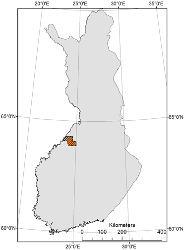
Fig. 1. The location of the study area.
The study area belongs entirely to the midboreal vegetation zone, and due to the flatness of the topography and humidity of the climate a considerable part of the area is covered by peatlands. The inventory area, defined by the area covered by airborne laser scanning, covers approximately 200 000 ha, of which approx. 149 000 ha is allocated to forestry land (mainly privately owned forests). Of the areas outside forestry land, 77.2% are agricultural lands, 4.5% consist of water bodies, 0.9% are allocated to peat extraction, and the remaining part is covered by artificial surfaces (traffic lanes, residential and other built-up areas). Based on the multi-source NFI of Finland, 64% of the forestry land is mineral land, 34% forested peatland (mainly pine bogs) and 2% open bog or mire. Furthermore, 47.5% of the forestry land is dominated by pine (Pinus silvestris), 3.4% by spruce (Picea abies) and 8.7% by broadleaved trees (mainly Betula pubescens and P. pendula), the rest is mixed forest with no dominant species or forest with low amount of growing stock (Tomppo et al. 2008; Tomppo et al. 2013). The principal silvicultural system has been even-aged management.
2.2 Field data
The field plots measured by the Northern Ostrobothnia Forest Centre (or ‘FC plots’) were selected via stratified cluster sampling. The stratification was based on earlier stand inventory data, and the stratification variables were forest site type, dominant tree species, proportion of dominant species, total basal area, and mean diameter of growing stock. The FC plots were measured as circular sample plots with a fixed radius of 5.64 m for seedling stands and 9 m for more mature stands. A plot was measured as a tally-tree plot on seedling stands approaching pulpwood size (5.64 m radius) and for more mature stands (9 m radius). On younger seedling stands, a plot was measured as a ‘stem number plot’, on which only stem number, mean diameter, and mean height by tree species group were assessed. On tally-tree plots, the diameter at breast height, tree species, and tree class (living/dead) of the tally trees were recorded. On the plots of 9 m radius, tally trees had a minimum diameter of 50 mm, while for the tally-tree plots on seedling stands, trees with heights of at least half the estimated mean height of the relevant species group were tallied. From each tree-species group (pines, spruces, and deciduous trees), one tree corresponding to the size of the basal-area-median-diameter tree was selected as a sample tree for which age and height too were measured (Heikkilä et al. 2010). The sample plots’ positions were measured via the global navigation satellite system (GNSS). A virtual reference station (VRS) system was used for correction of the measured locations to produce a sub-meter accuracy for the positioning. Co-ordinates of the individual tally and sample trees were not recorded. The plots were measured after the 2010 growing season.
The NFI data were selected from the field plots measured in 2006–2008 during the 10th inventory (NFI10) and in 2009–2010 during the 11th inventory (NFI11). The field sample plots were in clusters that were, as a rule, in a grid of 7 × 7 km. However, a quarter of the field plot clusters were permanent, and the grid of these clusters was different from the grid of the temporary clusters. In NFI10, 20% of the temporary clusters in South Finland were measured each year, in a five-year (2004–2008) inventory cycle. In North Finland, 25% of the temporary clusters were measured each year during the four-year (2005–2008) inventory cycle. Both in South and in North Finland, the permanent clusters were measured over four years, 25% of the clusters each year. In NFI11, the temporary clusters were relocated and their layout was modified slightly (fewer plots and more clusters). The permanent plots are being re-measured during the five-year period of NFI11 (2009–2013), 20% of them each year. North and South Finland are both divided further into three sampling zones. Most of the study area lies in North Finland in the sampling zone called Southern part of North Finland. A small part of the study areas lies in South Finland in the sampling zone called Central Finland. The distance between field plots in a cluster was 300 m in the both sampling zones. The plots were in either L-shaped or rectangular clusters, with the number of plots in each cluster being 9–14, depending on the sampling zone and the nature of the cluster (temporary or permanent). There was variation in the cluster form in the study data because the NFI sampling design varies by regions according to local conditions. Further, the design have been modified between inventories and we used data from both NFI10 and NFI11. The details of the sampling designs and field measurements are described in the field manuals (Valtakunnan metsien 2006; Valtakunnan metsien 2009).
The main features of the NFI and FC plot data are described in Table 1.
| Table 1. Main features of the two data types. | ||
| NFI | FC | |
| Plot type | Relascope | Variable radius circular |
| Radius/relascope factor | Central Finland factor 2 (max. radius 12.52 m), Southern North Finland factor 1.5 (max. radius 12.45 m). | Radius 5.64–9 m |
| Selection of plots | Systematic clustered sampling | Subjective stratified selection |
| Positioning | GPS (appr. 5 m accuracy) | GPS (appr. 1 m accuracy) |
| Average number of tally trees | 11.5 | 37.7 |
| Range of the number of tally trees per plot | 1–29 | 8–109 |
| Area represented by one plot a) | Central Finland 338 ha, Southern North Finland 417 ha | 318 ha (varies per inventory area) |
| Measurement years | 2006–2010 | 2010 |
| a) Expansion factor according to NFI11 design and 5 year data. | ||
A map of the sample plots’ positioning in the inventory area is presented in Fig. 2, along with forestry vs. non-forestry areas.
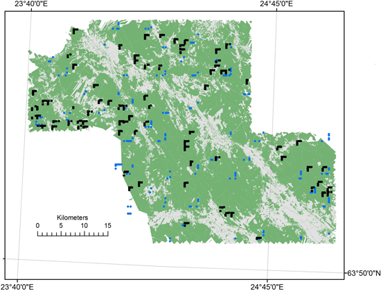
Fig. 2. The field sample layout in the study area defined by the laser scanning coverage (forestry land is shown in green, © MML, 2011). NFI plots = blue circles and FC plots = black rectangles.
In the NFI, tally trees are selected by means of a relascope, but there is a maximum distance for inclusion. In Southern North Finland, the basal area factor has been 1.5 and the maximum distance 12.45 m, while the basal area factor in Central Finland has been 2 and the maximum distance 12.52 m. For tally trees, the tree species, crown class, quality class, and diameter are registered. Every seventh tallied tree is a sample tree with more detailed measurements of, for example, height, diameter at six metres, and five-year increments of diameter and height.
An NFI plot in the study area was selected for a field check if the plot was within one forest stand. The field check was performed in autumn 2010 for finding plots whose centre point could still be found and in which tally trees had not been cut or fallen between the dates of the NFI measurements and ALS data collection. The positions of these plots, forming the NFI dataset, were then measured by means similar to those used for the FC plots.
In both field datasets, tree volumes were calculated with diameter and height as predictors (Laasasenaho 1982). Before that, the diameters of tally trees were updated for the date of the ALS data collection in line with diameter increment models in which the predicting variables were tree diameter and the stand variables basal area, mean age, and fertility class. The models for tree-species groups were constructed for increment percentage of diameter in the past five years, with the NFI10 sample trees in the area of the Northern Ostrobothnia Forest Centre for modelling data. Heights of tally trees with the updated diameters were predicted by a linear mixed-effects model (Eerikäinen 2009) that was localised with the sample trees of the dataset. In stem-number plots of FC data, mean heights and diameters were updated to the date of the collection of ALS data by means of simple models based on the average past annual increment of each measurement.
On tally-tree plots, mean diameter and mean height were calculated with basal area weighting. On FC plots, stand age was obtained as a weighted mean of the ages of the sample trees, weighted by the basal area sums of tally trees in the tree-species groups. On NFI plots, stand age estimated in the field was used. Stand ages were also adjusted to the date of the ALS data’s collection. In calculation of the per-hectare sum characteristics, the area of the inclusion zone for an NFI tree was defined by the diameter at measurement time, with the maximum distance for inclusion taken into account.
The basic field reference dataset consisted of the FC plots, used alone and in various combinations with the NFI plots in the estimation. The following field datasets were used in this study:
- FC, circular sample plots measured by the Northern Ostrobothnia Forest Centre: 468 plots
- NFIa, NFI plots measured in 2006–2010: 186 plots
- NFIb, NFI plots measured in 2008–2010 (older plots from 2006–07 were removed): 105 plots
- Replaced (an FC plot was replaced by an NFIb plot when one was available in the same stratum used for the allocation of the FC plots): 468 plots, where 103 of the FC plots were replaced with an NFIb plot
- NFIa+FC: 654 plots
- NFIb+FC: 573 plots
The statistics of the forest variables within the sample-plot combinations used as training or evaluation datasets are presented in Table 2. The distribution of volume classes within FC and NFI plots is illustrated in Fig. 3.
| Table 2. The statistics of the used sample plot combinations: mean, standard deviation (SD), maximum (Max). | |||||||
| Statistic | Dataset | H, m | D, cm | Vol, m3/ha | Pine, m3/ha | Spruce, m3/ha | Broadl., m3/ha |
| Mean | FC | 12.07 | 14.29 | 116.97 | 62.22 | 32.54 | 22.22 |
| Mean | Replaced | 12.18 | 14.68 | 116.87 | 64.25 | 31.32 | 21.3 |
| Mean | NFIa | 12.93 | 16.08 | 117.42 | 64.79 | 24.35 | 28.28 |
| Mean | NFIb | 13.54 | 17.12 | 117.72 | 68.99 | 22.88 | 25.86 |
| Mean | FC+NFIa | 12.32 | 14.8 | 117.1 | 62.95 | 30.21 | 23.94 |
| Mean | FC+NFIb | 12.34 | 14.81 | 117.11 | 63.46 | 30.77 | 22.88 |
| SD | FC | 4.94 | 6.4 | 82.61 | 58.78 | 54.65 | 33.48 |
| SD | Replaced | 4.94 | 6.51 | 81.86 | 60.28 | 53.6 | 33.55 |
| SD | NFIa | 3.27 | 4.36 | 70.54 | 55 | 45.23 | 46.92 |
| SD | NFIb | 3.18 | 4.42 | 67.08 | 56.7 | 37.23 | 42.88 |
| SD | FC+NFIa | 4.54 | 5.94 | 79.31 | 57.7 | 52.24 | 37.85 |
| SD | FC+NFIb | 4.7 | 6.18 | 79.93 | 58.41 | 52 | 35.38 |
| Max | FC | 22 | 33.6 | 428.6 | 329.1 | 321.3 | 233.4 |
| Max | Replaced | 22 | 33.6 | 428.6 | 329.1 | 321.3 | 265.8 |
| Max | NFIa | 20.4 | 27.6 | 347.6 | 255.3 | 333 | 265.8 |
| Max | NFIb | 20.4 | 27.6 | 282.7 | 255.3 | 161.6 | 265.8 |
| Max | FC+NFIa | 22 | 33.6 | 428.6 | 329.1 | 333 | 265.8 |
| Max | FC+NFIb | 22 | 33.6 | 428.6 | 329.1 | 321.3 | 265.8 |
| H = mean height, D = mean diameter, Vol. = total volume of growing stock, Pine/Spruce/Broadl. = volume of pine/spruce/broadleaved trees | |||||||
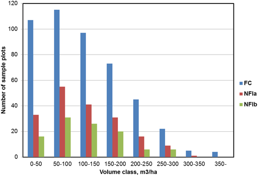
Fig. 3. The distribution of volume on the FC and NFI plots.
2.3 Remote-sensing data
2.3.1 Optical aerial imagery
The aerial images from the study area were acquired mainly in 2005–2009, although a small amount of the imagery from the middle of the study area was from 2004 and for a peripheral portion of the area from as early as 2002. Archived aerial photographs are often used in operational inventories, i.e. most up-to-date images available are utilised. Thus, the time span of the aerial imagery may be several years (as in this study). The aerial images were acquired mainly by means of digital camera sensor, with the exception of the images from 2002, which were scanned film photographs. The images were orthorectified with 50 cm ground resolution featuring green, red, and near-infrared bands.
2.3.2 ALS data
ALS data were acquired in May 2009, and the original customer was the National Land Survey of Finland, with a view to production of a digital terrain model of the area. Typically laser scanning for forestry purposes is carried out later in the summer, when vegetation is in full leaf. The scanning altitude was 1800 m, with a maximum zenith angle of 17° and side overlap of 20%. The density of returned pulses was 0.5407 per square metre. The attributes covered by the ALS data are listed in Table 3.
| Table 3. The attributes covered by the ALS data for lidar pulses. | |
| Column | Attribute description |
| 1 | x co-ordinate (X, EUREF-FIN Easting) |
| 2 | y co-ordinate (Y, EUREF-FIN Northing) |
| 3 | z co-ordinate (Z, height above sea level) |
| 4 | Intensity (I) |
| 5 | Classification (ground pulse / other) |
| 6 | Number of the return |
The ground elevation for each lidar point was estimated via spatial interpolation using two nearest-neighbour ground pulses and inverse distance weighting. The height above ground (H) was calculated for each lidar point as the difference between the z co-ordinate and the estimated ground level.
Along with the ALS point data, the ALS data were interpolated to a raster format for two output images: height and intensity. Based on earlier studies, for example the intensity texture has proved to be useful in the estimation of stand volume and biomass (e.g. Tuominen and Haapanen 2013). The pixel values of the height and intensity images were calculated via interpolation using inverse squared distance weighting of the two nearest ALS points of first echoes only. The power parameter of inverse distance weighting specifies how sample points are weighted, and a lower power tends to cause smoothing in the interpolated surface. Inverse squared distance weighting was judged as appropriate here, considering the density of lidar pulses and the shape of tree canopies. The interpolated images were resampled to the spatial resolution of the aerial images.
3 Methods
3.1 Extraction of remote-sensing features
The remote-sensing feature datasets were extracted from the ALS point data and aerial images, along with ALS height and intensity images. Features from the raster images were extracted for each sample plot from a 16.5 × 16.5 m square window whose centre was convergent with the sample-plot centre point. Features from ALS point data were extracted around the sample plot’s centre, with a circle of 9 m radius.
The following statistical and textural features were extracted from the aerial images and ALS height and intensity images:
- Averages of pixel values
- Standard deviations of pixel values
- Textural features based on co-occurrence matrices of pixel values (Haralick et al. 1973; Haralick 1979)
- Angular second moment
- Contrast
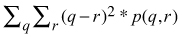
- Correlation
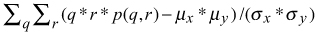
- Entropy
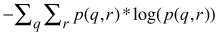
- Local homogeneity
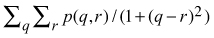
where
p(q,r) = M(q,r)/Nt
M(q,r) = the co-occurrence matrix of the requantified pixel values q and r
Nt = the total number of possible pairs in the image window
µx ,σx = the mean and standard deviation of the row sums of the co-occurrence matrix
µy ,σy = the mean and standard deviation of the column sums of the co-occurrence matrix
The textural features based on co-occurrence matrices of pixel values were extracted as average values for features calculated in four directions in the extraction window: horizontally (0° angle), vertically (90°), and diagonally (45° and 135°). Pixel lag of three metres was applied.
The following features were extracted from the ALS point data:
- Average value of H for vegetation pulses, first returns (m) (Packalén et al. 2009)
- Average value of H for vegetation pulses, last returns (m) (Packalén et al. 2009)
- Standard deviation of H for vegetation pulses, first returns (m) (Packalén et al. 2009)
- Standard deviation of H for vegetation pulses, last returns (m) (Packalén et al. 2009)
- H at which percentiles of vegetation pulses (0%, 5%, 10%, 20%, ..., 85%, 90%, 95%, 100%) accumulated, first returns (m) (Næsset 2004; Packalén and Maltamo 2006)
- H at which percentiles of vegetation pulses (0%, 5%, 10%, 20%, ..., 85%, 90%, 95%, 100%) accumulated, last returns (m) (Næsset 2004; Packalén and Maltamo 2006)
- Coefficient of variation of H for vegetation pulses, first returns (%) (Næsset 2004)
- Coefficient of variation of H for vegetation pulses, last returns (%) (Næsset 2004)
- Proportion of vegetation pulses, first returns (%) (Packalén et al. 2009)
- Proportion of vegetation pulses, last returns (%) (Packalén et al. 2009)
- Proportions of vegetation pulses having H above fraction* 0, 1, ..., 9 from all points, first returns (%) (Næsset 2004)
- Proportions of vegetation pulses having H above fraction* 0, 1, ..., 9 from all points, last returns (%) (Næsset 2004)
- Proportion of vegetation pulses having H greater than or equal to the corresponding percentile of H, (i.e., p20f is the proportion of points having H ≥ h20f), first returns (%), adapted from Packalén and Maltamo (2008)
- Proportion of vegetation pulses having H greater than or equal to the corresponding percentile of H, (i.e., p20l is the proportion of points having H ≥ h20l), last returns (%), adapted from Packalén and Maltamo (2008)
- Ratio of the number of vegetation pulses to the number of ground points, first returns (Packalén and Maltamo 2006)
- Ratio of the number of vegetation pulses to the number of ground points, last returns (Packalén and Maltamo 2006)
- Proportion of ground pulses, first returns (Packalén and Maltamo 2006)
- Proportion of ground pulses, last returns (Packalén and Maltamo 2006)
- Ratio of percentile (20%, 40%, 60% and 80%) of I to the 50% percentile of I, vegetation pulses, first returns (Vehmas et al. 2009)
- Ratio of percentile (20%, 40%, 60% and 80%) of I to the 50% percentile of I, vegetation pulses, last returns (Vehmas et al. 2009)
where
H = pulse height above ground
I = pulse intensity
vegetation pulse = pulse with H ≥ 2 m
ground pulse = other than vegetation pulse
* The range of H was divided into 10 fractions (0, 1, 2, …, 9), of equal distance.
All aerial image and ALS features were scaled to have a standard deviation of 1. This was done because the original features had very diverse scales of variation. Without scaling, variables with wide variation would have had greater weight in the estimation regardless of their correlation with the estimated forest attributes.
3.2 Estimation of forest attributes and selection of remote-sensing features
The k-nearest-neighbour (k-nn) method was used for estimation of the forest variables. The variables estimated were total volume of growing stock; the volumes of Scots pine, Norway spruce, and deciduous species; mean diameter; and mean height. Several values of k were tested in the estimation procedure. In the k-nn estimation (e.g., Kilkki and Päivinen 1987; Muinonen and Tokola 1990; Tomppo 1991; Tokola et al. 1996), the Euclidean distances between the sample plots were calculated in the n-dimensional feature space, where n represents the number of remote-sensing features extracted. The stand-variable estimates for the sample plots were calculated as weighted averages for the stand variables of the k nearest neighbours (see Eq. 1). Weighting by inverse Euclidean distances raised to the power g in the feature space was applied (see Eq. 2) to diminish the bias of the estimates (Altman 1992). The optimal value for g was tested in the estimation.

where
ŷ = estimate for the variable y
yi = measured value of the variable y on the ith nearest neighbouring plot
wi = 
di = Euclidean distance (in the feature space) to the ith nearest neighbour plot
k = number of nearest neighbours
g = parameter for adjusting the progression of weight with increasing distance
The accuracy of the estimates was calculated via leave-one-out cross-validation through comparison of the estimated forest variable values with the measured values (ground truth) of the field plots. The accuracy of the estimates was measured in terms of absolute and relative root mean square error (RMSE %) (see Eq. 3) and bias statistics.

where
RMSE = 
yi = observed value of the variable y on plot i
ŷi = estimated value of the variable y on plot i
![]() = mean of the observed values
= mean of the observed values
n = number of plots
The remote-sensing datasets encompassed, in total, 122 ALS and aerial-image features. In a large feature set, some features are less relevant and some may be highly correlated, such as the similar features calculated from the first and last returns in the ALS data. Therefore, selection of the features and their weighting were performed with a genetic-algorithm-based approach, implemented in the language R (R Development Core Team 2010) by means of the Genalg package (Willighagen 2005). The evaluation function of the genetic algorithm was employed to minimise the sum of weighted RMSEs and absolute biases of k-nn estimates in leave-one-out cross-validation. In the minimisation, the weights for the target variables mean height, mean diameter, total volume of growing stock, volume of pine, volume of spruce, and volume of deciduous species were 15%, 10%, 40%, 10%, 10%, 15%, respectively.
Features to be used with all datasets were selected with the combined dataset FC+NFIb. Weights for the selected features were then sought separately for each reference dataset. In the feature selection, the population consisted of 400 binary chromosomes and the number of generations was 250. We carried out 20 feature-selection runs to find the feature set that returned the best evaluation value. In the feature weights’ selection, floating-point chromosomes (values in the range 0–1) were used and the number of generations was increased to 400. Otherwise the procedure was similar to that in the feature selection. The values of parameters k (Eq. 1) and g (Eq. 2) were selected through a few test runs. The parameter k was set to 6, and g was set to 2.7.
4 Results
The RMSE statistics showed that the FC plots performed better alone than in combination with the NFI plots in the k-nn estimation. There was a clear improvement in the estimates when the older NFI plots, measured in 2004–2005, were excluded from the estimation. In estimation of stand mean height, diameter, or total volume of growing stock, the FC plots yielded the best estimation results. For estimation of the growing-stock volumes for the tree-species groups, the combination of FC plots and NFI plots from 2006–2008 (NFIb) showed the best estimation results. When the estimation results were calculated separately for FC and NFIb plots with the combined set (FC+NFIb) as the reference set, the results were substantially better for the FC plot set than for the NFIb plot set.
Mean stand height was the most accurate variable to estimate (relative RMSE = 8.67% with FC plots). The relative RMSEs of stand mean-diameter estimates were between 15.64% (FC) and 17.12% (NFIb). The RMSE of the total-volume estimates was 21.74% for the FC plots and 27.77% for the NFI plots. The volumes of tree species were the most difficult variables to estimate, with the relative RMSEs varying between 47.98% and 86.45% in estimates for the FC plots with the FC+NFIb set used as reference, and 47.96–109.35% in estimation for the NFIb plots with FC+NFIb as reference. Thus, the combination of the FC and NFI plots improved the estimation of tree-species volumes. The estimates of pine volume were considerably more accurate than the estimates for spruce and broadleaf species, as pine was the dominant tree species in the study area and had the highest average volume on both NFI and FC plots.
With the estimation option in which FC plots were replaced with NFI plots of similar forest class (‘Replaced’), the result was a deterioration in the estimation accuracy. This was true in the case wherein Replaced was used as both the estimation target and the reference and also when Replaced was used as the reference and FC as the target.
The difference in estimation accuracy between FC and NFI plots (measured by the ratio of their relative RMSEs) was greatest for the volume of spruce and the smallest with the volume of broadleaf trees. This finding is consistent with the fact that the average volume of spruce was much higher on the FC plots than the NFI plots (where the average volume of broadleaf trees was higher than the equivalent figure for spruce). For the rest of the forest variables, the difference in estimation accuracy was smallest for stand height and total volume. The bias of the estimates was otherwise very small, except for the cases wherein the reference and target set of plots were different. When estimates for NFIb plots were generated with FC+NFIb as the reference set, the greatest bias resulted, for all forest variables.
The RMSE and bias statistics from cross-validation for the tested forest variables and various combinations of field plots are presented in Tables 4a–4f. The list of selected features and their correlations with the estimated forest variables are presented in Appendices 1 and 2.
| Table 4a. Accuracy of the mean-height estimates. | ||||
| Reference | Target | RMSE (m) | RMSE (%) | Bias (m) |
| FC | FC | 1.05 | 8.67 | 0.01 |
| Replaced | FC | 1.11 | 9.20 | 0.05 |
| FC+NFIb | FC | 1.08 | 8.93 | 0.02 |
| Replaced | Replaced | 1.17 | 9.56 | 0.00 |
| FC+NFIb | NFIb | 1.42 | 10.49 | –0.12 |
| FC | FC+NFIb | 1.12 | 9.10 | –0.01 |
| FC+NFIb | FC+NFIb | 1.15 | 9.31 | –0.01 |
| FC+NFIa | FC+NFIa | 1.18 | 9.57 | 0.00 |
| Table 4b. Accuracy of the mean-diameter estimates. | ||||
| Reference | Target | RMSE (cm) | RMSE (%) | Bias (cm) |
| FC | FC | 2.23 | 15.64 | –0.01 |
| Replaced | FC | 2.33 | 16.29 | 0.29 |
| FC+NFIb | FC | 2.26 | 15.83 | 0.14 |
| Replaced | Replaced | 2.39 | 16.27 | –0.01 |
| FC+NFIb | NFIb | 2.93 | 17.12 | –0.87 |
| FC | FC+NFIb | 2.38 | 16.10 | –0.18 |
| FC+NFIb | FC+NFIb | 2.40 | 16.20 | –0.05 |
| FC+NFIa | FC+NFIa | 2.35 | 15.88 | 0.00 |
| Table 4c. Accuracy of the total-volume estimates. | ||||
| Reference | Target | RMSE (m3/ha) | RMSE (%) | Bias (m3/ha) |
| FC | FC | 25.43 | 21.74 | 0.02 |
| Replaced | FC | 27.70 | 23.68 | –0.18 |
| FC+NFIb | FC | 26.75 | 22.87 | –0.97 |
| Replaced | Replaced | 26.72 | 23.64 | 0.05 |
| FC+NFIb | NFIb | 32.69 | 27.77 | 4.82 |
| FC | FC+NFIb | 27.33 | 23.34 | 0.94 |
| FC+NFIb | FC+NFIb | 27.93 | 23.85 | 0.09 |
| FC+NFIa | FC+NFIa | 29.41 | 25.12 | 0.01 |
| Table 4d. Accuracy of the pine volume estimates. | ||||
| Reference | Target | RMSE (m3/ha) | RMSE (%) | Bias (m3/ha) |
| FC | FC | 30.41 | 48.87 | 1.56 |
| Replaced | FC | 30.84 | 49.56 | 1.75 |
| FC+NFIb | FC | 29.85 | 47.98 | 0.55 |
| Replaced | Replaced | 30.90 | 48.09 | 0.92 |
| FC+NFIb | NFIb | 33.08 | 47.96 | 4.95 |
| FC | FC+NFIb | 32.02 | 50.46 | 2.27 |
| FC+NFIb | FC+NFIb | 30.47 | 48.01 | 1.36 |
| FC+NFIa | FC+NFIa | 32.58 | 51.76 | 1.54 |
| Table 4e. Accuracy of the spruce volume estimates. | ||||
| Reference | Target | RMSE (m3/ha) | RMSE (%) | Bias (m3/ha) |
| FC | FC | 23.73 | 72.92 | –0.33 |
| Replaced | FC | 24.01 | 73.8 | –0.86 |
| FC+NFIb | FC | 23.16 | 71.16 | –1.00 |
| Replaced | Replaced | 23.53 | 75.12 | 0.06 |
| FC+NFIb | NFIb | 20.41 | 89.22 | 3.75 |
| FC | FC+NFIb | 23.95 | 77.84 | 0.57 |
| FC+NFIb | FC+NFIb | 22.68 | 73.7 | –0.13 |
| FC+NFIa | FC+NFIa | 24.12 | 79.85 | –0.12 |
| Table 4f. Accuracy of the broadleaf volume estimates. | ||||
| Reference | Target | RMSE (m3/ha) | RMSE (%) | Bias (m3/ha) |
| FC | FC | 19.72 | 88.75 | –1.21 |
| Replaced | FC | 21.01 | 94.56 | –1.06 |
| FC+NFIb | FC | 19.21 | 86.45 | –0.52 |
| Replaced | Replaced | 20.29 | 95.29 | –0.94 |
| FC+NFIb | NFIb | 28.27 | 109.35 | –3.89 |
| FC | FC+NFIb | 21.6 | 94.37 | –1.90 |
| FC+NFIb | FC+NFIb | 21.16 | 92.47 | –1.14 |
| FC+NFIa | FC+NFIa | 22.12 | 92.40 | –1.40 |
5 Discussion
The results of this study showed that use of the NFI plots in addition to the FC plots generally improved the volume estimates by species group (although the bias of spruce volume estimates seemed to increase for some reason) but not the estimates of total volume. It can be assumed that the main reason for the latter is the difference in the sample-plot type. The inclusion area of the relascope (Bitterlich) sample plot does not match the area of RS feature extraction: small trees are measured only near the plot centre while large trees are included from further off the plot centre than on the FC plots. Therefore, relascope plots are not so well suited to use as a field reference for ALS data. Furthermore, as the FC data were collected on the basis of a priori data, it can be assumed that said dataset covers the variation in the study area better than the NFI set does (see Fig. 3). The slight improvement in volume estimates by species when the NFI plots are introduced in the reference data indicates that the number of plots in the FC plot dataset was not adequate for all proportions of species. This result encourages further development of utilisation of NFI plots in management-planning inventories. However, it should be noted that interpretation of small differences or even fair comparison of data sets is difficult based on leave-one-out cross-validation and heuristic feature or feature weight selection with possible overfitting problems (see Packalén et al. 2012).
The main obstacle to utilisation of NFI plots in classification of ALS data for management-planning inventories is the size of an NFI plot for small trees. The plots should be larger than they are in the current design for small trees. If the cost of measuring many small trees in the NFI is considered too high, the use of a smaller relascope factor in combination with a maximum radius for sampling of the tally trees would improve the feasibility of NFI plots as reference data, since the sample plot would then be more representative, especially for young stands. A variable-radius plot, possibly with several small sub-plots for the smallest trees, could also be an efficient solution for tree measurements. On the other hand, selection of any sample-plot design is a difficult compromise, since the NFI measurements are aimed at optimisation of the cost–inventory accuracy trade-off at larger area level, for which a fixed-radius sample plot would be less optimal.
Perhaps the most realistic way of using NFI plots in combination with ALS- and aerial-image-based forest inventory is to utilise an existing systematic sample of NFI plots as a starting point that would be supplemented with sample plots allocated to forest classes without NFI plots in order to cover the relevant variation of forest variables in the inventory area. This kind of layout was simulated in this study through use of the dataset Replaced as the reference in estimation of the variables of the FC dataset. As noted above, in the ‘Results’ section, this resulted in a decline in estimation accuracy in comparison to the option wherein only FC plots were utilised. Therefore, if such a system is considered desirable, the usability of the NFI plots for this purpose should be improved via revision to the measurement design.
One option for the utilisation of NFI plots might be to apply stratified sampling in allocation of the plots, to make sure that the sample covers all relevant forest classes in the inventory area. Even if the bulk of the NFI plots were selected systematically, further or different measurements more suitable for reference plots could be assigned to a certain number of the NFI plots on the basis of pre-stratification. The fact that introducing NFI plots to the reference data improved estimates of volumes by species indicates that the original FC reference data did not include enough observations to cover the species-mixture combinations properly. The stratification parameters or the allocation of plots to the various strata must be revised. In a practical forest-inventory application in an area with enough NFI plots, an additional option would be to use a systematic NFI sample as an initial set of reference plots, accompanied by additional reference plots allocated on the basis of later stratification of NFI plots in relation to the relevant forest categories (those requiring extra observations).
The usability of NFI plots may improve in the near future as the use of modern tree callipers that measure also tree distance from the plot centre becomes fully implemented. When the tree distance is known, the tree data can be resampled to match the ALS data. Furthermore, the use of electronic tree callipers will reduce the cost of a tree measurement in relation to the ‘fixed costs’ of measuring one plot. Thereby, the proportion of small trees on the NFI plots can be increased without too great an increase to the total cost of the inventory.
In many countries, including Finland, NFI data with exact coordinates is not available to public due to protection of land owners’ privacy. This limits the possibilities to use NFI data in remote sensing studies. However, it is possible to develop a web service to combine the plot data and remote sensing data without revealing the coordinates to the data users.
As described above, the inventory unit in the Forest Centre’s method has been fixed to a grid-cell size of 16 × 16 m. Forest attributes for forest stands or compartments are aggregated from attributes of these grid cells. In some previous studies (e.g., van Aardt et al. 2006; Hyvönen et al. 2005; Tuominen and Haapanen 2011), segments have been used as inventory and estimation units. These segments can be small and complicated in size. Therefore, 16 × 16 cells might be too large and many of them may be crossed by boundary lines of segments. Accordingly, reducing the size of the cells in the grid might lead to more reliable results. Also, in this case, the flexible use of varying sample-plot radius to match the resolution of the remote-sensing material is a key component. However, it must be noted that the smaller the units are, the more accurate the location of the sample plots and geo-referenced remote-sensing material must be. A number of studies focusing on field observations (in appropriate quantities) for ALS-based forest inventories have noted that quite a low number of reference plots suffices when those plots are carefully selected (e.g., Gobakken and Næsset 2008; Junttila et al. 2008; Maltamo et al. 2011). The above-mentioned studies point to even 60–100 field reference plots as enough for reaching relatively high estimation accuracy for variables such as the total volume of growing stock, and the addition of further plots does not significantly improve the estimation accuracy.
Also in the study of Maltamo et al. (2009) fixed radius plots performed better that the relascope plot for classification of ALS data. The study showed also that even a relatively dense systematic sampling, far more intensive than used in real NFI in Finland, does not guarantee a sample that covers well the variation of the population.
It is typical in the case of operational forest inventories for many of the inventory variables to be estimated (among them the volumes of various tree species), and the estimation problem is more complicated. For example, the selection of remote-sensing features is a compromise between the estimation accuracies of several inventory variables. In such a case, it is very likely that a significantly higher number of field reference plots is going to be required for sufficiently covering the relevant variation over the variables of interest. Nonetheless, it is evident that the set of FC plots measures up to the inventory standards in the study area.
Because of the relatively small size of FC management-planning inventory campaigns, the number of NFI plots is low in a typical area of ALS inventory. One solution to this problem would be the utilisation of NFI plots that lie outside the ALS inventory area (on the assumption that ALS and aerial-image features are available also for these plots, although from separate rather than simultaneous scanning). This raises the question of the general compatibility of remote-sensing data features. Currently, local field reference data are utilised in FC inventories. The commensurability of ALS features across geographical areas has been examined in several studies (e.g., Lefsky et al. 2002; Lefsky et al. 2005; Suvanto and Maltamo 2010). Lefsky et al. (2002, 2005) have suggested that, with respect to coniferous forests, there might exist a distinct universal relationship between the ALS features and forest structure, making it possible to generalise the reference data over various types of geographical areas (assuming similar laser-scanning parameters). Therefore, utilisation of sample plots from different geographical areas, covered by separate laser scanning, might not be a problem, at least within the same vegetation zone. Features in aerial photographs often show variation that is caused by factors other than the properties of the objects in the image. The aerial-image pixel values are affected by the illumination conditions, the viewing geometry, atmospheric conditions, and factors such as land cover or vegetation type (e.g., Jackson et al. 1990; Li and Strahler 1992; Pellikka et al. 2000; Lillesand et al. 2004). Therefore, it is characteristic of aerial images that their spectral properties in particular are heterogeneous even in a small area, whereas the textural features should be more uniform over different image-acquisition operations (e.g., Tuominen and Pekkarinen 2005).
References
Altman N.S. (1992). An introduction to kernel and nearest-neighbor nonparametric regression. The American Statistician 46: 175–185.
Eerikäinen K. (2009). A multivariate linear mixed-effects model for the generalization of sample tree heights and crown ratios in the Finnish National Forest Inventory. Forest Science 55(6): 480–493.
Gobakken T., Næsset E. (2008). Assessing effects of laser point density, ground sampling intensity, and field plot sample size on biophysical stand properties derived from airborne laser scanner data. Canadian Journal of Forest Research 38: 1095–1109. http://dx.doi.org/10.1139/X07-219.
Gregoire T.G., Ståhl G., Naesset E., Gobakken T., Nelson R., Holm S. (2011). Model-assisted estimation of biomass in a lidar sample survey in Hedmark County, Norway. Canadian Journal of Forest Research 41: 83–95. http://dx.doi.org/10.1139/X10-195.
Haralick R. (1979). Statistical and structural approaches to texture. In: Proceedings of the IEEE 67(5): 786–804. http://dx.doi.org/10.1109/PROC.1979.11328.
Haralick R., Shanmugan K., Dinstein I. (1973). Textural features for image classification. IEEE Transactions on Systems, Man and Cybernetics, SMC-3(6): 610–621. http://dx.doi.org/10.1109/TSMC.1973.4309314.
Heikkilä J., Ärölä E., Kilpiäinen S. (2010). Kaukokartoitusperusteisen metsien inventoinnin koealojen maastotyöopas (versio 0.8). Tapio ja Suomen Metsäkeskus. 21 p.
Holmgren J., Jonsson T. (2004). Large scale airborne laser-scanning of forest resources in Sweden. International Archives of Photogrammetry, Remote Sensing and Spatial Information Sciences. Volume XXXVI, Part 8/W2: 157−160.
Hyvönen P., Pekkarinen A., Tuominen S. (2005). Segment-level stand inventory for forest management. Scandinavian Journal of Forest Research 20: 75–84. http://dx.doi.org/10.1080/02827580510008220.
Jackson R.D., Teillet P.M., Slater P.N., Fedosejevs G., Jasinski M.F., Aase J.K., Moran M.S. (1990). Bidirectional measurements of surface reflectance for view angle corrections of oblique imagery. Remote Sensing of Environment 32: 189–202. http://dx.doi.org/10.1016/0034-4257(90)90017-G.
Junttila V., Maltamo M., Kauranne T. (2008). Sparse Bayesian estimation of forest stand characteristics from ALS. Forest Science 54: 543–552.
Kilkki P., Päivinen R. (1987). Reference sample plots to combine field measurements and satellite data in forest inventory. Department of Forest Mensuration and Management, University of Helsinki, Research Notes 19: 210–215.
Köhl M., Magnussen S., Marchetti M. (2006). Sampling methods, remote sensing and GIS multiresource forest inventory. Tropical Forestry. Springer. ISBN-13 978-3-540-32571-0. http://dx.doi.org/10.1007/978-3-540-32572-7_6.
Koivuniemi J., Korhonen K.T. (2006). Inventory by compartments. In: Kangas A., Maltamo M. (eds.). Forest inventory. Methodology and applications. Managing Forest Ecosystems, vol. 10. Springer. p. 271–278.
Laasasenaho J. (1982). Taper curve and volume functions for pine, spruce and birch. Communicationes Instituti Forestalis Fenniae 108.
Lefsky M.A., Cohen W.B., Harding D.J., Parker G.G., Acker S.A., Gower S.T. (2002). Lidar remote sensing of aboveground biomass in three biomes. Global Ecology and Biogeography 11(5): 393–400. http://dx.doi.org/10.1046/j.1466-822x.2002.00303.x.
Lefsky M., Hudak A., Cohen W., Acker S.A. (2005). Geographic variability in lidar predictions of forest stand structure in the Pacific Northwest. Remote Sensing of Environment 95: 532–548. http://dx.doi.org/10.1016/j.rse.2005.01.010.
Li X., Strahler A.H. (1992). Geometric-optical bidirectional reflectance modeling of the discrete crown vegetation canopy: Effect of crown shape and mutual shadowing. IEEE Transactions on Geoscience and Remote Sensing 30: 276–292. http://dx.doi.org/10.1109/36.134078.
Lillesand T.M., Kiefer R.W., Chipman J.W. (2004). Remote sensing and image interpretation. Fifth edition. John Wiley & Sons, Inc. 763 p.
Maltamo M., Packalen P., Suvanto A., Korhonen K., Mehtätalo L., Hyvonen P. (2009). Combining ALS and NFI ground truth data for forest management planning – a case study in Kuortane, Western Finland. European Journal of Forest Research 128: 305–317. http://dx.doi.org/10.1007/s10342-009-0266-6.
Maltamo M., Bollandsås O.M., Næsset E., Gobakken T., Packalén P. (2011). Different plot selection strategies for field training data in ALS-assisted forest inventory. Forestry 84: 23–31. http://dx.doi.org/10.1093/forestry/cpq039.
Muinonen E., Tokola T. (1990). An application of remote sensing for communal forest inventory. In: Proceedings from SNS/IUFRO Workshop: The Usability of Remote Sensing for Forest Inventory and Planning (conference held in Umeå, Sweden, on 26–28 February). Remote Sensing Laboratory, Swedish University of Agricultural Sciences, Report 4: 35–42.
Næsset E. (2004). Practical large-scale forest stand inventory using a small footprint airborne scanning laser. Scandinavian Journal of Forest Research 19: 164–179. http://dx.doi.org/10.1080/02827580410019544.
Næsset E., Gobakken T., Bollandsås O.M., Gregoire T.G., Nelson R., Ståhl G. (2013). Comparison of precision of biomass estimates in regional field sample surveys and airborne LiDAR-assisted surveys in Hedmark County, Norway. Remote Sensing of Environment 130: 108–12. http://dx.doi.org/10.1016/j.rse.2012.11.010.
Packalén P., Maltamo M. (2006). Predicting the plot volume by tree species using airborne laser scanning and aerial photographs. Forest Science 52(6): 611–622.
Packalén P., Maltamo M. (2008). Estimation of species-specific diameter distributions using airborne laser scanning and aerial photographs. Canadian Journal of Forest Research 38: 1750–1760. http://dx.doi.org/10.1139/X08-037.
Packalén P., Suvanto A., Maltamo M. (2009). A two stage method to estimate species-specific growing stock. Photogrammetric Engineering and Remote Sensing 75(12): 1451–1460. http://dx.doi.org/10.14358/PERS.75.12.1451.
Packalén P., Temesgen H., Maltamo M. (2012). Variable selection strategies for nearest neighbor imputation methods used in remote sensing-based forest inventory. Canadian Journal of Remote Sensing 38(5): 1–13. http://dx.doi.org/10.5589/m12-046.
Pellikka P., King D.J., Leblanc S.G. (2000). Quantification and reduction of bidirectional effects in aerial CIR imagery of deciduous forest using two reference land surface types. Remote Sensing Reviews 19(1–4): 259–291. http://dx.doi.org/10.1080/02757250009532422.
R Development Core Team. (2010). R: a language and environment for statistical computing. R Foundation for Statistical Computing, Vienna. ISBN 3-900051-07-0. http://www.R-project.org/. [Cited 4 June 2012].
Ståhl G., Holm S., Gregoire T.G., Gobakken T., Naesset E., Nelson R. (2011). Model-based inference for biomass estimation in a Lidar sample survey in Hedmark County, Norway. Canadian Journal of Forest Research 41: 96–107. http://dx.doi.org/10.1139/X10-161.
Suvanto A., Maltamo M. (2010). Using mixed estimation for combining airborne laser scanning data in two different forest areas. Silva Fennica 44(1): 91–107.
Tokola T., Pitkänen J., Partinen S., Muinonen E. (1996). Point accuracy of a non-parametric method in estimation of forest characteristics with different satellite materials. International Journal of Remote Sensing 17(12): 2333–2351. http://dx.doi.org/10.1080/01431169608948776.
Tomppo E. (1991). Satellite image-based national forest inventory of Finland. International Archives of Photogrammetry and Remote Sensing 28: 419–424.
Tomppo E., Haakana M., Katila M., Peräsaari J. (2008). Multi-source national forest inventory – methods and applications. Managing Forest Ecosystems 18. Springer. 374 p.
Tomppo E., Gschwantner T., Lawrence M., McRoberts R. (eds.). (2010). National Forest Inventories. Pathways for common reporting. Springer. http://dx.doi.org/10.1007/978-90-481-3233-1.
Tomppo E., Katila M., Mäkisara K., Peräsaari J. (2013). The multi-source National Forest Inventory of Finland – methods and results 2009. Metlan työraportteja / Working Papers of the Finnish Forest Research Institute 273. 216 p.
Tuominen S., Haapanen R. (2011). Comparison of grid-based and segment-based estimation of forest attributes using airborne laser scanning and digital aerial imagery. Remote Sensing 3(5) (Special Issue ‘100 Years ISPRS – Advancing Remote Sensing Science’): 945–961.
Tuominen S., Haapanen R. (2013). Estimation of forest biomass by means of genetic algorithm-based optimization of airborne laser scanning and digital aerial photograph features. Silva Fennica 47(1) 902. http://dx.doi.org/10.14214/sf.902.
Tuominen S., Pekkarinen A. (2005). Performance of different spectral and textural aerial photograph features in multi-source forest inventory. Remote Sensing of Environment 94(2): 256–268. http://dx.doi.org/10.1016/j.rse.2004.10.001.
Valtakunnan metsien 10. inventointi (VMI10) (2006). Maastotyön ohjeet 2006. Koko Suomi. Metsäntutkimuslaitos, Helsinki. 107 p. http://www.metla.fi/ohjelma/vmi/vmi10-maasto-ohje-06.pdf. [Cited 15 May 2012].
Valtakunnan metsien 11. inventointi (VMI11) (2009). Maastotyön ohjeet 2009. Koko Suomi. Metsäntutkimuslaitos, Vantaa, Finland. 122 p. http://www.metla.fi/ohjelma/vmi/vmi11-maasto-ohje09-2p.pdf. [Cited 15 May 2012].
van Aardt J.A., Wynne R.H., Oderwald R.G. (2006). Forest volume and biomass estimation using small-footprint lidar-distributional parameters on a per-segment basis. Forest Science 52: 636–649.
Vehmas M., Eerikäinen K., Peuhkurinen J., Packalén P., Maltamo M. (2009). Identification of boreal forest stands with high herbaceous plant diversity using airborne laser scanning. Forest Ecology and Management 257: 46–53. http://dx.doi.org/10.1016/j.foreco.2008.08.016.
Willighagen E. (2005). Genalg: R based genetic algorithm. R package version 0.1.1.
Wulder M.A., White J.C., Nelson R.F., Næsset E., Ørka H.O., Coops N.C., Hilker T., Bater C.W., Gobakken T. (2012). Lidar sampling for large-area forest characterization: a review. Remote Sensing of Environment 121: 196–209. http://dx.doi.org/10.1016/j.rse.2012.02.001.
Total of 46 references
Appendices
| Appendix 1. List of features from the remote-sensing dataset that got selected for k-nn estimation. |
| Average of pixel values on near-infrared band of aerial image (mean_nir) |
| Average of pixel values in intensity image (mean_i) |
| Angular second moment on red band of aerial image (asmavg_r) |
| Entropy in height image (entavg_h) |
| Average value of H for vegetation pulses, first returns (m) (havgf) |
| H at which 40% of vegetation pulses accumulated, first returns (m) (h40f) |
| H at which 70% of vegetation pulses accumulated, first returns (m) (h70f) |
| H at which 90% of vegetation pulses accumulated, first returns (m) (h90f) |
| H at which 100% of vegetation pulses accumulated, first returns (m) (h100f) |
| H at which 5% of vegetation pulses accumulated, last returns (m) (h5l) |
| H at which 90% of vegetation pulses accumulated, last returns (m) (h90l) |
| Proportion of vegetation pulses having H above fraction 4 from all points, first returns (%) (d4f) |
| Proportion of vegetation pulses having H above fraction 0 from all points, last returns (%) (d0l) |
| Proportion of vegetation pulses having H above fraction 2 from all points, last returns (%) (d2l) |
| Proportion of vegetation pulses having H greater than or equal to the 60% percentile of H from all points, first returns (%) (p60f) |
| Ratio of the 80% percentile of I to the 50% percentile of I, vegetation pulses, last returns (i80l) |
| Appendix 2. Correlations between remote-sensing features selected for estimation and field attributes on dataset FC+NFIb (for abbreviations of features, see Appendix 1). | ||||||
| Feature | H | D | Vol | Pine | Spruce | Broadl. |
| mean_nir | –0.43 | –0.47 | –0.29 | –0.27 | –0.37 | 0.34 |
| mean_i | –0.68 | –0.59 | –0.68 | –0.42 | –0.32 | –0.38 |
| asmavg_r | –0.28 | –0.28 | –0.17 | –0.22 | 0.05 | –0.1 |
| entavg_h | 0.92 | 0.85 | 0.79 | 0.47 | 0.44 | 0.36 |
| havgf | 0.94 | 0.88 | 0.84 | 0.56 | 0.37 | 0.42 |
| h40f | 0.94 | 0.88 | 0.85 | 0.52 | 0.41 | 0.45 |
| h70f | 0.96 | 0.91 | 0.84 | 0.48 | 0.47 | 0.42 |
| h90f | 0.97 | 0.92 | 0.83 | 0.46 | 0.5 | 0.39 |
| h100f | 0.96 | 0.92 | 0.82 | 0.44 | 0.51 | 0.37 |
| h5l | 0.75 | 0.7 | 0.61 | 0.59 | 0.07 | 0.3 |
| h90l | 0.97 | 0.92 | 0.83 | 0.46 | 0.48 | 0.39 |
| d4f | 0.74 | 0.65 | 0.81 | 0.63 | 0.32 | 0.33 |
| d0l | 0.8 | 0.74 | 0.81 | 0.4 | 0.6 | 0.29 |
| d2l | 0.82 | 0.75 | 0.82 | 0.5 | 0.53 | 0.27 |
| p60f | 0.11 | 0.1 | 0.08 | 0.15 | –0.07 | 0.05 |
| i80l | 0.49 | 0.44 | 0.3 | 0.1 | 0.08 | 0.39 |
