Annika Kangas  ,
Terje Gobakken,
Stefano Puliti,
Marius Hauglin,
Erik Naesset
,
Terje Gobakken,
Stefano Puliti,
Marius Hauglin,
Erik Naesset
Value of airborne laser scanning and digital aerial photogrammetry data in forest decision making
Kangas A., Gobakken T., Puliti S., Hauglin M., Naesset E. (2018). Value of airborne laser scanning and digital aerial photogrammetry data in forest decision making. Silva Fennica vol. 52 no. 1 article id 9923. https://doi.org/10.14214/sf.9923
Highlights
- Airborne laser scanning (ALS) and digital aerial photogrammetry (DAP) are nearly equally valuable for harvest scheduling decisions even though ALS data is more precise
- Large underestimates of stand volume are most dangerous errors for forest owner because of missed cutting probabilities
- Relative RMSE of stand volume and the mean volume in a test area explain 77% of the variation between the expected losses due to errors in the data in the published studies
- Increasing the relative RMSE of volume by 1 unit, increased the losses in average by 4.4 € ha–1.
Abstract
Airborne laser scanning (ALS) has been the main method for acquiring data for forest management planning in Finland and Norway in the last decade. Recently, digital aerial photogrammetry (DAP) has provided an interesting alternative, as the accuracy of stand-based estimates has been quite close to that of ALS while the costs are markedly smaller. Thus, it is important to know if the better accuracy of ALS is worth the higher costs for forest owners. In many recent studies, the value of forest inventory information in the harvest scheduling has been examined, for instance through cost-plus-loss analysis. Cost-plus-loss means that the quality of the data is accounted for in monetary terms through calculating the losses due to errors in the data in the forest management planning context. These costs are added to the inventory costs. In the current study, we compared the losses of ALS and DAP at plot level. According to the results, the data produced using DAP are as good as data produced using ALS from a decision making point of view, even though ALS is slightly more accurate. ALS is better than DAP only if the data will be used for more than 15 years before acquiring new data, and even then the difference is quite small. Thus, the increased errors in DAP do not significantly affect the results from a decision making point of view, and ALS and DAP data can be equally well recommended to the forest owners for management planning. The decision of which data to acquire, can thus be made based on the availability of the data on first hand and the costs of acquiring it on the second hand.
Keywords
forest inventory;
value of information;
uncertainty;
remote sensing;
cost-plus-loss;
data quality
-
Kangas,
Natural Resources Institute Finland (Luke), Bioeconomy and environment, P.O. Box 68, FI-80170 Joensuu, Finland
E-mail
annika.kangas@luke.fi
- Gobakken, Faculty of Environmental Sciences and Natural Resource Management, Norwegian University of Life Sciences, P.O. Box 5003, NO-1432 Ås, Norway E-mail terje.gobakken@nmbu.no
- Puliti, Faculty of Environmental Sciences and Natural Resource Management, Norwegian University of Life Sciences, P.O. Box 5003, NO-1432 Ås, Norway E-mail stefano.puliti@nibio.no
- Hauglin, Faculty of Environmental Sciences and Natural Resource Management, Norwegian University of Life Sciences, P.O. Box 5003, NO-1432 Ås, Norway E-mail marius.hauglin@nmbu.no
- Naesset, Faculty of Environmental Sciences and Natural Resource Management, Norwegian University of Life Sciences, P.O. Box 5003, NO-1432 Ås, Norway E-mail erik.naesset@nmbu.no
Received 30 November 2017 Accepted 19 January 2018 Published 24 January 2018
Views 138897
Available at https://doi.org/10.14214/sf.9923 | Download PDF

1 Introduction
During the last decade, airborne laser scanning (ALS) has been the most important data acquisition method for forest management inventories both in Finland and Norway (Næsset 2007; Packalen and Maltamo 2007). The possibility of collecting three-dimensional (3D) data using digital aerial photogrammetry (DAP) during relatively frequent aerial image acquisition campaigns has in recent years been under active research and development. DAP data are usually markedly cheaper than ALS data, provided that a digital terrain model is already available from previous ALS campaigns. Typically forest parameters (e.g. volume, basal area, height, diameter) estimated from DAP data have been less accurate than those estimated from ALS data (Bohlin et al. 2012; Vastaranta et al. 2013; Straub et al. 2013; Rahlf et al. 2014; Yu et al. 2015), but some studies have demonstrated that similar accuracies may be obtained with the two data sources (Gobakken et al. 2015; Tuominen et al. 2017; Puliti et al. 2017).
Any non-trivial decision typically includes uncertainty concerning the prevailing state of nature (Hirshleifer and Riley 1979). The decision maker can then either make an optimal choice between different alternatives with the current information or reduce the uncertainty by collecting more information. Value of information (VOI) in decision making (ex ante) can hereby be defined as the difference between the expected value of this choice with and without the additional information (Hirshleifer and Riley 1979; Lawrence 1999; Kangas 2010). The VOI of given data acquisition methods thus determines if the difference in the quality of information for different methods is important in practise: the higher the difference in VOI between methods, the more important the difference is in practise.
The problem can also be looked at from a different perspective by analysing the losses due to sub-optimal decisions. Then, the VOI comes from the reduced expected losses when additional information comes available. This approach has been more commonly used in forestry, where different inventory methods have been compared to each other using a so-called cost-plus-loss (CPL) analysis. In CPL, the total costs of an inventory consist of the inventory costs and the losses due to sub-optimal decisions, and the inventory method having the lowest total costs is defined as best (Hamilton 1978; Burkhart et al. 1978).
Most of the applications of CPL in forestry have dealt with defining the expected losses from a given data acquisition method, such as sampling-based forest inventory, traditional visual forest inventory, photo interpretation-based forest inventory, and ALS-based forest inventory (Holmström et al. 2003; Eid et al. 2004; Mäkinen et al. 2010; Borders et al. 2010). In some of the analyses, also other sources of error, such as error in the estimation of diameter distributions has been included (Bergseng et al. 2015). In most cases, analysis has been carried out by assuming that the utility of the decision maker only consists of the net present value (NPV) of the decision without any area-level constraints, such as even-flow or end inventory constraints. The time horizon has varied from 10 years (Holmström et al. 2003) to 100 years (Eid et al. 2004) and the interest rate from 2% to 4%. The calculations have been carried out with local planning systems, with either stand-level or single-tree level growth models.
In addition, the studies have been carried out for areas with differences in characteristics such as proportion of mature stands and number of plots or stands. Finally, some of the studies have been carried out using real forest data (Eid et al. 2004) with only one realization of each method for each plot/stand, while in other cases the analysis has been carried out using simulated data (Mäkinen et al. 2010). The results from the CPL analyses carried out so far show large variations. The losses due to the imperfect data have varied from around 13 € ha–1 (Eid et al. 2004) to 470 € ha–1 (Mäkinen et al. 2010). There can be many reasons for this variation, and if the causes of differences in results can be identified, it may be easier to interpret the results and generalize from previous and current findings.
The aim of this study was to analyse the importance of the difference in data quality between DAP data and ALS data when used for forest management planning. The study was carried out by quantifying and analysing the monetary losses due to the errors in the forest estimates obtained with the two different data acquisition methods. We also analysed how the length of planning period affects the expected losses. Finally, we carried out a meta-analysis of the losses observed in the CPL studies so far, in order to detect the reasons for the large variation of losses between different studies.
2 Material
2.1 Study area
The study was conducted in the municipalities of Gran, Lunner, and Jevnaker (Fig. 1), southeastern Norway, as part of an operational forest management inventory going on in the area. The total inventory area was 726 km2, located at 114–810 m a.s.l., and the main tree species in the area are Norway spruce (Picea abies (L.) Karst.) and Scots pine (Pinus sylvestris L.).
The study took advantage of existing operational stand-based forest inventories conducted 10–15 years ago. The stand values were prorated and the stands were divided into three initial strata according to tree species, age, and site quality information from the previous inventory. The three strata used in this study were stratum A: mature spruce-dominated stands on good sites; stratum B: mature pine-dominated stands on good sites; stratum C: young forest above 8 m in mean height. Good site quality was assigned to sites with interpreted H40 site index values greater than 12.5. The H40 site index is defined by dominant height (hdom) and average age of the dominant trees. hdom is defined as the mean height of the 100 largest trees per hectare according to diameter at breast height (dbh). The specific values of the H40 index relate to hdom at an index age of 40 years (Tveite 1977; Braastad 1980). Plots with broadleaves as the main tree species were not included in this study.
2.2 Field data
Field data were collected during summer and fall 2016 and consisted of 314 circular field plots of size 250 m2. The plots were grouped into clusters of nine plots. In each cluster, the plots were located in a 3 × 3 grid with 250 m between the plot centres. The minimum distance between clusters was 1.5 km, but not all clusters were measured. The final sample therefore cannot be considered a probability sample. Not all plots in every cluster were measured due to harvests since the previous inventory and location of plots outside forest area. Initial plot coordinates were imported into hand held Global Navigation Satellite System (GNSS) receivers and the plot positions were located by navigating to the plot centres in the field.
The position of each plot centre was recorded with sub-meter accuracy using Topcon HiPer V and Topcon Legacy-E dual-frequency receivers observing pseudorange and carrier phase of both the global positioning system and the global navigation satellite system. Collection of data lasted from 11 to 99 minutes with 35 minutes in average, with a 1s logging rate. The recorded GNSS data were postprocessed with correction data from a base station. The distance from the plots to the base station varied from 1.3 km to 22.5 km with 13.4 km as the average. The horizontal errors of the final coordinates reported by the Magnet Tools postprocessing software (Topcon Positioning Systems Inc.) were at maximum 82 cm with an average value of 3 cm.
On each plot, dbh (for trees with dbh > 6 cm) was callipered and tree heights were measured on sample trees. The sample trees were selected with a probability proportional to stem basal area. The number of sample trees per plot ranged from 1 to 29 with an average of 9.6.
The heights were measured with a Vertex hypsometer. For the remaining trees, heights were predicted using height-dbh models by Fitje and Vestjordet (1977) and Vestjordet (1968). The volume of each sample tree was predicted using species-specific volume models with dbh and either measured height or predicted height as independent variables (Braastad 1966; Brantseg 1967; Vestjordet 1967). The ratio of the mean volume estimates for trees with predicted heights and the mean volume estimates for trees with measured heights was used to adjust the former volume estimates. Final height estimates for trees without height measurements were obtained by inverting the species-specific volume models to predict height, using the estimated volume and measured dbh as independent variables. The ground reference mean height of each plot was computed as the so-called Lorey’s mean height (hL), i.e. mean height weighted by basal area (Table 1). Dominant height of each plot was computed as arithmetic mean of the two largest trees according to diameter. Mean plot diameter was computed as mean basal area diameter (dg) from diameter of all callipered trees. Stem number was computed as number of trees per hectare (N). Plot basal area (G) was computed as basal area per hectare from the breast height diameter measurements. Total plot volume (V) was computed as the sum of the individual tree volumes.
| Table 1. Summary of the data from the 314 field plot (250 m2). | |||
| Characteristic | Minimum | Maximum | Mean |
| hL (m) | 7.03 | 32.51 | 16.41 |
| hdom (m) | 8.96 | 33.60 | 19.39 |
| dg (cm) | 8.3 | 44.2 | 17.8 |
| N (ha–1) | 160 | 3120 | 1246 |
| G (m2 ha–1) | 3.32 | 78.42 | 28.52 |
| V (m3 ha–1) | 14.91 | 992.12 | 242.93 |
| Tree species distribution | |||
| Spruce (%) | 0 | 100 | 69 |
| Pine (%) | 0 | 100 | 22 |
| Broadleaved species (%) | 0 | 83 | 9 |
| hL = Lorey’s mean height, hdom = dominant height, dg = mean basal area diameter, N = stem number, G = basal area, V = volume. | |||
2.3 Remotely sensed data
The remotely sensed data consisted of wall-to-wall DAP data and wall-to-wall ALS data. Both data types involve point clouds with x, y and z coordinates. In ALS data these point clouds represent the whole vertical structure of the trees, as the laser beams penetrate the canopy, while in DAP the points all represent the surface. Thus, both give information on the density of the stand and the height, but only ALS data can describe the canopy structure.
2.3.1 Digital aerial photogrammetry data
674 spectral images from 22 flight lines were acquired with a Vexcel UltraCamEagle and a Vexcel UltraCamXp sensor on 9 June and 15 August 2015, respectively, by Terratec AS, Norway. The side and forward overlaps between images were 20% and 60%, respectively. In the current study only colour infra-red (RGBI) 8 bit digital imagery was used as these were the only products that could be delivered by the contractor. The images were acquired from a mean flying altitude of 4260 m and 3580 m above ground level for the UltraCamEagle and UltraCamXp, respectively. The different altitudes were used to account for different sensor image resolutions and to ensure the same ground sample distance of 25 cm for both acquisitions.
The sensor location and orientation during image acquisition were recorded using a GNSS and an inertial navigation system. A photogrammetric point cloud and canopy height model were constructed from the aerial images using SURE Photogrammetric software (Rothermel et al. 2012) which adopts a matching algorithm similar to Semi-Global Matching (SGM) proposed by Hirschmuller (2008) and Rothermel et al. (2012). The software was chosen over alternative ones because of the ability to efficiently process large datasets and the ability to ensure larger height variations compared to other photogrammetric software (Haala 2014). It is likely that larger height variations can provide more valuable information on the forest canopy.
The input data for the generation of the dense point cloud were: 1) non-orthorectified 8 bit RGBI UltraCam imagery; and 2) the aerial triangulation provided by the data vendor. The processing was performed with default settings and resulted in the production of a point cloud with a point density of approximately 33.4 points m–2. Because of the differences in the two sensors used and different flight altitudes, the processing was performed separately for the two different areas. A Dell PowerEdge R730 2.2 Ghz 128 GB RAM server was used for the processing and the overall processing time was 80 hours.
2.3.2 Airborne laser scanning data
ALS data were collected in two data collections 2–10 May and 11–20 June 2015 using two Leica ALS70 sensors as part the Norwegian “National Detailed Elevation Model” program. The ALS instruments were operated at a minimum altitude above ground level of 1108 m. The flight speed was 77 m s−1. The pulse repetition frequency was 273 kHz and the maximum scan angle was ±16°. The point density was approximately of 14.9 points m−2. Pre-processing of the ALS data was carried out by the contractor (Terratec AS, Norway). This included the computation of planimetric coordinates, ellipsoid height values, and point cloud classification into ground and non-ground echoes according to the proprietary algorithm implemented in the Terrascan software (Soininen 2016). A triangulated irregular network (TIN) model was then created by linear interpolation from the ground-classified points. The acquisitions in May and June were under leaf-off and leaf-on conditions, respectively. The Leica ALS70 sensors are capable of recording an unlimited number of echoes per pulse. In the current study, we used the three echo categories classified as “single”, “first of many”, and “last of many”. The “single” and “first of many” echoes were pooled into one dataset denoted as “first” echoes, and correspondingly, the “single” and “last of many” echoes were pooled into a dataset denoted as “last” echoes.
2.4 Computations and modelling
Heights above the ground surface were calculated for all first and last ALS echoes and the DAP point cloud by subtracting the ALS TIN heights from the height values of all echoes and points recorded. The ALS echoes and DAP points were extracted for each field plot. Separate distributions were derived from the first and last ALS echoes and from the DAP dataset. A threshold of 1.3 m above ground was used to define canopy echoes. Below this height, ALS echoes and DAP points were considered to have been reflected from shrubs, grass, or ground, i.e. a non-tree objects. Height variables including maximum value (hmax), mean value (hmean), coefficient of variation (hcv), and percentiles at 10% intervals (h0, h10, …, h90) were derived from the canopy echoes. Furthermore, several measures of canopy density were derived. The calculation of canopy density was carried out for 10 different vertical layers of equal height (Næsset 2004b). The height of each layer was defined as one tenth of the distance between the 95 percentile and the lowest canopy height, i.e. 1.3 m (Gobakken et al. 2012). Canopy densities were then computed as the proportions of ALS echoes or DAP points above fraction #0, 1, …, 9 to total number of echoes or points and denoted d0, d1, …, d9, respectively. Two dummy variables were also introduced to assess seasonal differences in the remotely sensed data. The value for the first dummy variable was set to 0for the plots covered by the leaf-off acquisition and 1 for the plots covered by the leaf-on acquisition. In a similar way, the second dummy variable was used to discriminate between acquisitions performed with each of the two cameras.
The variables derived from the remotely sensed data were related to the ground values for the field plots using stratum-specific multiple regression analysis for ALS and DAP datasets. In the regression analysis, multiplicative models were constructed as linear regressions using logarithmic transformations of the variables as this has shown to be suitable for modelling of e.g. mean height, stem number, and volume by others (Næsset 2002b). Both first and last echo variables were used when the models were developed by means of ALS data.
The standard least-squares method and stepwise selection with a significance level of 0.05 was applied to select variables to be included in the final models. Selection of predictor variables was performed using a best subset regression procedure implemented in the “leaps” package (Lumley and Miller 2017) in R, constrained to include a maximum of five predictors in the models. To avoid overfitting and multicollinearity, the models were selected using the Bayesian information criterion and variance inflation factors were kept below five. An empirical ratio estimator for bias correction proposed by Snowdon (1991) was employed when converting the logarithmic predictions to arithmetic scale; the proportional bias in logarithmic regression being estimated from the ratio of the mean of the observed values to the mean of the back-transformed predicted values. Predictions were finally corrected by multiplying them by the estimated ratio. The R2 value was calculated in the original scale as the square of Pearson’s correlation coefficient between the field and predicted values. The fitted models were evaluated based on the R2 values.
No independent plot data were available to assess the accuracy of the constructed regression models at a spatial scale equivalent to the size of the field plots (250 m2). Leave-one-plot-out cross validation was therefore used to assess the accuracy. For each stratum consisting of n training plots, one of the training plots was removed from the dataset at a time, and the selected models were fitted to the data from the n–1 remaining plots. The studied biophysical forest variables (volume, basal area, Lorey’s height, dominant height, stem number, mean diameter) were then estimated for the removed field plot. This procedure was repeated until predicted values were obtained for all field plots. The accuracy of the predictions was assessed by the relative mean difference and the relative RMSE calculated on the original scale (Eq. 1 and 2):
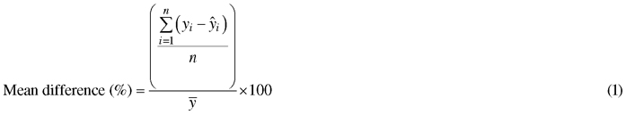
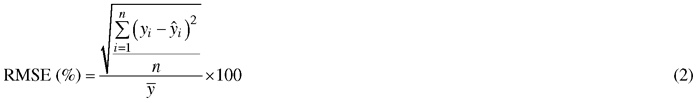
where n is the number of field plots, yi is the ground value for plot i, ![]() is the predicted value using the model, and
is the predicted value using the model, and ![]() is the mean of the ground values. Accuracy of the three most important variables in ALS and DAP data, respectively, are presented by the stratum in Table 2.
is the mean of the ground values. Accuracy of the three most important variables in ALS and DAP data, respectively, are presented by the stratum in Table 2.
| Table 2. The accuracy of the resulting data in the three strata and overall, for Lorey’s mean height, stem number and volume in leave-one-plot-out cross validation. | |||||||||
| Lorey’s mean height | |||||||||
| ALS | DAP | ||||||||
| Stratum | N | R2 | Mean dif. (%) | RMSE (%) | R2 | Mean dif. (%) | RMSE (%) | ||
| 1 | 78 | 0.88 | –0.1 | 6.9 | 0.80 | 0.0 | 6.7 | ||
| 2 | 106 | 0.86 | 0.0 | 7.7 | 0.85 | 0.0 | 8.0 | ||
| 3 | 130 | 0.90 | 0.0 | 7.4 | 0.85 | 0.0 | 9.0 | ||
| Total | 314 | 0.91 | –0.04 | 7.42 | 0.90 | 0.0 | 7.95 | ||
| Stem number | |||||||||
| ALS | DAP | ||||||||
| Stratum | N | R2 | Mean dif. (%) | RMSE (%) | R2 | Mean dif. (%) | RMSE (%) | ||
| 1 | 78 | 0.69 | 0.1 | 28.1 | * | 0.51 | –0.1 | 35.6 | * |
| 2 | 106 | 0.56 | 0.0 | 35.4 | 0.43 | 0.0 | 39.9 | ||
| 3 | 130 | 0.65 | 0.0 | 24.2 | * | 0.57 | 0.0 | 26.8 | * |
| Total | 314 | 0.64 | 0.05 | 28.34 | 0.52 | –0.02 | 32.72 | ||
| Volume | |||||||||
| ALS | DAP | ||||||||
| Stratum | N | R2 | Mean dif. (%) | RMSE (%) | R2 | Mean dif. (%) | RMSE (%) | ||
| 1 | 78 | 0.82 | 0.3 | 20.8 | 0.71 | 0.0 | 25.7 | ||
| 2 | 106 | 0.89 | 0.0 | 19.2 | 0.79 | –0.1 | 26.6 | ||
| 3 | 130 | 0.92 | 0.0 | 18.3 | 0.84 | –0.1 | 25.6 | ||
| Total | 314 | 0.91 | 0.08 | 20.78 | 0.81 | –0.05 | 27.14 | ||
| * Dummy variables representing airborne laser scanning (ALS) and digital aerial photogrammetry (DAP) acquisitions significant at 5%-level. | |||||||||
3 Methods
3.1 Simulation of treatment schedules for the plots
The large-scale forestry scenario model, GAYA, based on simulation of treatments for each plot (Hoen and Eid 1990; Hoen and Gobakken 1997) was used to calculate the losses due to imperfect data. GAYA is based on an area-based stand growth model with dg and hL as the basic entities, and N as the scaling factor. The simulations were based on dg increment models (Blingsmo 1984), hdom development models for spruce (Tveite 1977), pine (Tveite 1976), and birch (Braastad 1977), and a mortality model developed for spruce but applied also for pine and birch (Braastad 1982). Timber values were estimated from gross price models (Blingsmo and Veidahl 1992) and harvest costs from models based on a tariff agreed upon by employers’ and employees’ organizations in Norway. An annual real rate of discount of 3% was applied. Projections were performed for 20 periods of 5 yrs and all harvests were assumed to take place in the middle of a period. The variables G, Hdom, and N were estimated by the two remote sensing-based inventory methods and used as input to GAYA. Other input variables such as site index and age were kept constant when comparing the methods.
3.2 Calculation of the losses
In order to calculate the losses, both the true and erroneous data must be available for the area in question. The field sample is considered as ground truth, and the data obtained from ALS and DAP are assumed to be the erroneous data. The optimal treatment schedules were calculated using the field data, ALS data, and finally the DAP data. Then, the true NPVs of the schedules selected for ALS and DAP data were calculated based on the field data. The difference between the true optimum calculated with the field data and the value of the optimum with the erroneous data is the estimate of the loss (Ståhl et al. 1994; Eid et al. 2004; Fig. 2).
The losses were further divided into the 5-year periods. If either the true optimal treatment or the sub-optimal treatment occurred in a given period, the loss was included as a loss for that period. It means that the error could be either harvesting too early (the harvest was suggested for the erroneous data but not for true data) or too late (the harvest was suggested in the optimal data but not in the erroneous data), and the period was defined based on which of these occurred first. In later periods only new errors were counted, i.e. neither the erroneous or true data suggested harvest in any of the earlier periods. All the losses were assigned according to the first treatment. In some stands also second harvest is possible, but in the second harvest the inventory errors from the beginning are not relevant any more.
Finally, the losses were grouped using a regression tree approach (Breiman et al. 1984; rpart package in R). While it is not possible to accurately predict them at stand level, we assumed that it is possible to define groups where the accurate forest information is most important, i.e. where the losses are greatest.
3.3 Meta-analysis
The meta-analysis was based on five studies, with two or more methods compared in one or more test data sets (Table 3). From each of the studies, the available information was collected. Unfortunately, the reported characteristics between the studies varied quite much. The mean loss, mean volume in the field data, and relative standard error of volume and number of stems were the most frequently reported characteristics. The relative standard error of ALS volumes for Eid et al. (2004) was calculated from Næsset (2002, 2004). Studies where these characteristics could not be found, were excluded from the analysis.
| Table 3. The results of five cost-plus-loss analysis, and the mean volume, relative standard error of volume, and stem number in these studies. | ||||||||
| S | A | Method | R | M | Loss (€ ha–1) | Mean Vol | RMSE (%) Vol | RMSE (%) N |
| 1 | a | ALS | 3 | 0 | 13.4 | 219 | 12.0 | 20.6 |
| 1 | a | MPI | 3 | 0 | 50.9 | 219 | NA | 30.4 |
| 1 | b | ALS | 3 | 0 | 13.3 | 224 | 12.1 | 15.7 |
| 1 | b | MPI | 3 | 0 | 46.3 | 224 | NA | 36 |
| 2 | c | ALS_MV | 3 | 1 | 327.7 | 209 | 9.9 | 37.1 |
| 2 | c | ALS_DD | 3 | 1 | 60.7 | 209 | 14.1 | 33.2 |
| 2 | c | ITC | 3 | 1 | 78.9 | 209 | 33.4 | 62.8 |
| 2 | c | SITC | 3 | 1 | 109.2 | 209 | 28 | 26.7 |
| 3 | d | Plot10 | 2 | 1 | 9.02 | 272 | 9 | 8 |
| 3 | d | Plot5 | 2 | 1 | 13.95 | 272 | 10 | 12 |
| 3 | d | ImpLS | 2 | 1 | 80.65 | 272 | 18 | 19 |
| 3 | d | ImpLa | 2 | 1 | 107.82 | 272 | 18 | 21 |
| 3 | d | ImpSp | 2 | 1 | 194.03 | 272 | 33 | 33 |
| 3 | d | Plot10 | 4 | 1 | 1.89 | 272 | 9 | 8 |
| 3 | d | Plot5 | 4 | 1 | 3.46 | 272 | 10 | 12 |
| 3 | d | ImpLS | 4 | 1 | 36.29 | 272 | 18 | 19 |
| 3 | d | ImpLa | 4 | 1 | 79.29 | 272 | 18 | 21 |
| 3 | d | ImpSp | 4 | 1 | 201.90 | 272 | 33 | 33 |
| 4 | e | visual | 3 | 1 | 469.95 | 57.5 | 60.4 | 105.2 |
| 4 | e | ALS1 | 3 | 1 | 412.11 | 42.2 | 44.6 | 73.3 |
| 4 | e | ALS2 | 3 | 1 | 448.26 | 48.7 | 59.9 | 84.6 |
| 5 | f | ALS | 3 | 0 | 76.26 | 242.9 | 20.8 | 28.4 |
| 5 | f | DAP | 3 | 0 | 82.79 | 242.9 | 27.2 | 32.8 |
| Study (S) is 1: Eid et al. 2004; 2: Bergseng et al. 2015; 3: Duvemo et al. 2007; 4: Mäkinen et al. 2010; 5: the current study. Area (A) is a: Våler; b: Krødsherad; c: Aurskog; d: Remningstorp; e: simulated data; f: the current study area. Method is ALS: area-based laser scanning; MPI: manual photo interpretation; ALS_MV: area-based laser scanning with mean values; ALS_DD: area-based laser scanning with diameter distribution; ITC: individual tree crowns; SITC: semi-individual tree crowns; Plot5: 5 field plots; Plot10: 10 field plots; ImpLS: imputation using laser scanning and satellites; ImpLa: imputations using laser scanning; ImpSp: using satellite, visual assessment in field; ALS1 and ALS2: denote two different data sets for which the errors are simulated. R = interest rate (%). M is 0: stand-level growth model; 1: single-tree growth model. | ||||||||
From these reported values, the relationship between the mean loss and characteristics of the test were analysed using linear regression analysis. We analysed which of the reported characteristics of the studies could statistically significantly explain the variation in the observed losses.
4 Results
4.1 Cost-plus loss analysis
While the relative standard errors of V, G, and N clearly differed between data acquired using ALS and DAP, the differences in the losses calculated for the whole 100-year planning horizon were relatively small. The mean loss with DAP data was 82.79 € ha–1, while it was 76.26 € ha–1 for the ALS data. Thus, the DAP produced on average 8.5% larger losses (Table 4). Altogether, the losses per ha were quite small. The maximum losses were exactly the same for DAP and ALS.
| Table 4. The main features of observed losses with airborne laser scanning (ALS) and digital aerial photogrammetry (DAP). | ||
| Loss (€ ha–1) | ||
| DAP | ALS | |
| Min. | 0.00 | 0.00 |
| Median | 0.00 | 0.00 |
| Mean | 82.79 | 76.26 |
| Max. | 1841.62 | 1841.62 |
In most of the plots, no losses were observed (e.g. the median was 0for both methods), and in vast majority of the plots they were fairly small (Fig. 3). However, non-zero losses were observed in 43.6% for ALS (137 plots) and 43.3% for DAP (136 plots). Of these, in 105 cases losses were observed with both methods, and about 30 cases where such that losses were observed only with one of the methods (Fig. 4). The correlation between the losses in these two methods was 75%.
The errors in the first period accounted for almost 50% of the total losses (30–35 € ha–1), while the losses rapidly decreased over time (Fig. 5). After the 7th period, no additional losses were observed, meaning that all the stands were treated within the first seven periods. Obviously, the inventory errors do not have an effect on model-predicted stand development after a clear-cut. Also discounting reduces the effect of the losses over time. When only the first period was accounted for, the mean loss with ALS was 34.57 € ha–1 and with DAP 33.31 € ha–1. With ALS, erroneous decisions in the first period were observed in 30 plots and with DAP in 26 plots. However, the decision was not the same for these two methods for eight of the plots in the first period.
When the ALS losses of the first period were grouped based on the true volume in the plots using a regression tree, a two-level tree gave a very clear grouping (Fig. 6). In ALS data, the losses for plots with volume smaller than 392 m3 ha–1 were on average 9.6 € ha–1, for plots with volume larger than 597 m3 ha–1 they were 0€ ha–1, and for the volume range between 392 m3 ha–1 and 597 m3 ha–1, the losses were largest, i.e. 223 € ha–1 (Table 5).
| Table 5. The mean and maximum loss and the standard deviation of losses in the three volume groups for the first period and the whole planning horizon in € ha–1 with airborne laser scanning (ALS) and digital aerial photogrammetry (DAP). | |||||||
| Method | Group m3 ha–1 | First period | Planning horizon | ||||
| Mean | Max | Sd | Mean | Max | Sd | ||
| ALS | V < 392 | 9.62 | 451.88 | 47.75 | 52.71 | 914.43 | 132.02 |
| 392 < V < 597 | 223.16 | 1841.62 | 522.27 | 262.56 | 1841.62 | 530.56 | |
| V > 597 | 0.0 | 0 | 0 | 0.0 | 0 | 0 | |
| DAP | V < 392 | 6.02 | 508.09 | 37.90 | 57.11 | 1183.05 | 145.80 |
| 392 < V < 597 | 238.79 | 1841.62 | 526.19 | 285.92 | 1841.62 | 542.46 | |
| V > 597 | 0 | 0 | 0 | 0 | 0 | 0 | |
When this same grouping was used for DAP, the results were similar (Table 5). For the group with smallest volume the losses were even lower on average, but for the intermediate volumes a bit larger. The same analysis was carried out as a function of the error in the volume estimate. The errors in volume varied from an overestimate of 174 m3 ha–1 to 279 m3 ha–1 underestimate for ALS (mean 0.2 m3 ha–1), and from 211 m3 ha–1 of overestimate to 331 m3 ha–1 underestimate for DAP (mean –0.1 m3 ha–1). However, if the error was smaller than an underestimate of 43 m3 ha–1 (ALS) or 31 m3 ha–1 (DAP) the losses were very small. For those cases, the estimated volume was either overestimated or only slightly underestimated (Fig. 7). The largest losses were observed when the volumes were very substantially underestimated (error was larger than 117 m3 ha–1 (ALS) or 167 m3 ha–1 (DAP)).
When the losses from the entire planning horizon were considered (Table 5), the last group still showed zero losses. These stands were clear-cut in the beginning of the planning horizon. No other losses were observed later on, as the characteristics of the regenerated areas did not involve inventory errors. The losses from the first group increased to about 52–58 € ha–1, as in these stands treatment decisions were carried out in later periods. The losses in the intermediate volume group also increased a bit, but the largest losses were already observed in the first five years. When calculated for the original three strata formed for modelling purposes on the basis of maturity and tree species, the mean losses in the first period were 88, 72, and 72 € ha–1 for ALS and 91, 71, and 86 € ha–1 for DAP, indicating that DAP performed slightly worse in the young sites than ALS.
If the data were to be used only for the first 5-yr period, the difference between ALS and DAP method would be 1.26 € ha–1, with DAP showing slightly smaller losses. In practise, the difference would nevertheless be negligible. Based on this analysis, there is no reason for collecting the more expensive ALS data for forest management planning, as DAP data is equally well suited. If the data were to be used for 10 years, ALS showed a smaller loss of 1.13 € ha–1 compared to DAP (52.15 € ha–1 versus 51.02 € ha–1). Only if the data were to be used for 15 years or longer, ALS was superior (Fig. 5). Even then, the difference was negligible.
4.2 Meta-analysis
The meta-analysis was carried out using the available information in Table 3. The losses observed in different studies and with different methods were related to the used interest rate, growth model type, the mean volume of the case study data and the relative RMSE of volume and stem number estimates in each of the studies. The correlation of the observed mean loss with the mean volume in the datasets was –0.82, with the relative standard error for volume 0.83, and with the relative standard error for stem number 0.86 (Fig. 8).
The correlation between the relative standard error of volume and the loss would have been even larger, if one of the observations, namely ALS_MV (Bergseng et al. 2015) were excluded. In that case, values for volume, basal area, mean diameter and mean height were first predicted using ALS, and a diameter distribution was predicted using those, while in ALS_DD method of the same study the diameter distribution was directly predicted using ALS. The resulting relative standard error of volume was small, but the losses in € ha–1 large. Thus, in this method, the calculation of diameter distribution introduced additional errors into the analysis, as with the other methods used in Bergseng et al. (2015) the results were well in line with this meta-analysis.
Together the first two characteristics explained about 77% of the variation of losses between the different studies (Table 6). Both variables were significant with α = 0.05. Interest rate or the standard error of stem number were not significant predictors given that the relative RMSE of volume and mean volume were already included.
| Table 6. The performance of the model predicting the mean loss in the case studies. | ||||
| Estimate | Std. Error | t value | Pr(>|t|) | |
| Intercept | 238.7186 | 119.2609 | 2.002 | 0.0606 |
| Mean Volume | –0.9457 | 0.3686 | –2.565 | 0.0195 |
| Relative RMSE, volume | 4.3930 | 1.7947 | 2.448 | 0.0249 |
We also tested whether the type of growth models had an effect on the losses. In this study and in Eid et al. (2004) a stand level growth model was used, but in the other studies of the meta-analysis single tree growth models were used. Thus, we tested a dummy variable for the single tree models for the meta-analysis model. Introducing the dummy showed an increase of 69 € ha–1 when using a single tree model, but the effect was not statistically significant (p = 0.11). The non-significant result is likely due to the small amount of observations in the meta-study. This result indicates that had we used a simulator with single-tree models, slightly different results would have been obtained. However, based on the meta-analysis model, in mature stands the quality of decisions (i.e. the expected losses) can be predicted very well with RMSE of the volume in the data used for those decisions. On average, increasing the relative RMSE of volume by 1 unit, would increase the losses by 4.4 € ha–1, Ceteris paribus (i.e. with the same simulator and same test data). In this study, the RMSE increased from ALS to DAP by 6.4 units, which would give an average difference of 28.1 € ha–1. The observed difference was 6.53, meaning the difference here was smaller than on average in the published studies..
5 Discussion
Use of ALS in the forest management inventory has been a great success by producing high-quality data compared to the traditional method based on visually interpreted aerial photographs. In recent years, the DAP has been proved to be a very promising alternative to the ALS (Gobakken et al. 2015; Tuominen et al. 2017; Puliti et al. 2017). In all studies the accuracy of the DAP has been lower than that of ALS, but in the most recent studies the difference has been quite small. In the current study, we aimed at analysing if the difference in the accuracy is of importance in monetary terms for the forest owners’ decision making.
According to our results, the difference in accuracy is negligible from the forest owner’s point of view, especially if the data will be used for at most 10 years. If the data are to be used for a longer time period, ALS performed better. In the current management inventory and planning regime, however, it is not likely that collected data would actually be used for a longer time period than 10 years, and it is likely that new or modified methods (e.g. higher ALS pulse densities) offering higher accuracies would be available by then. Therefore, we can recommend that the DAP data can be utilized in forest planning interchangeably with the ALS data, i.e. the forest owners should choose the type of data based on availability and the cost of the data. While the DAP showed very good performance in this analysis, one should keep in mind that this is only a single individual case study, and the results are based on 314 plots only, so generalization should be done with caution. However, the fact that the results are well in line with previous studies, gives some confidence in generality of our result.
In this case study, only large underestimates seemed to contribute to large losses in monetary terms. Such underestimates are likely to postpone the harvest decisions markedly. Thus, from the forest owner’s perspective, underestimates seem much more problematic than overestimates. Kangas et al. (2011) also noted that underestimates and overestimates have a different importance from a decision making point of view. The most problematic cases would be stands with high volumes that are substantially underestimated.
In this study, we used plots rather than stands in the comparison. In the stand level, the RMSE of volume would likely be smaller, and thus also the resulting losses would be likely to be smaller. It is also likely that at stand level, the probability of very large underestimates or overestimates would be smaller. However, when related to the observed relative RMSE, the results observed here are in line with the other studies carried out.
The losses observed in the cost-plus-loss analyses carried out in recent studies have shown quite large variation. In the meta-analysis, we concluded that the accuracy of the tested data had a very clear role in contributing to the losses, and so does the characteristics of the test area in question. The more mature the stands are, the smaller are the losses observed (Eid et al. 2004; Mäkinen et al. 2010). On the other hand, the length of the planning horizon that varied from 10 to 100 years in the studied cases, had only a minor effect on the results. Obviously, the most substantial losses are encountered already in the first years of using a plan, and the last years do not add much to the losses. Likewise, the role of interest rate was quite small.
The use of single-tree versus stand level growth models was statistically insignificant, but it should be kept in mind when interpreting the results of future studies. It is reasonable to expect that the growth model type would have a significant effect in a larger meta-dataset, if such were available. Even if the model type had a significant effect on the losses, the differences observed between methods in each case study are accurate, if we assume that the effect of model type changes only the level of the losses (i.e. the intercept of the meta-analysis model) rather than the slope. In that case, the model type has no effect on the comparison. However, it would also mean that observed losses between case studies with a different model types are not comparable unless the model type is accounted for.
The losses in younger stands have been analysed in a relatively few papers. In Mäkinen et al. (2010), also younger stands were involved, and the losses were markedly larger than in the other studies. Therefore, more research should be devoted to the analysis of required quality in such stands. For instance in Kangas et al. (2014), additional measurements needed in each stand were selected simultaneously with the selection of the optimal treatment options for the same stands. In that study, even if the inventory was assumed to cost 18 € ha–1, measuring the young and well growing stands proved to be profitable, but measuring the mature stands was not. However, in that study the data were assumed to be used for more than 40 years. This indicates that the length of planning horizon would also have a larger effect in young stands than in mature stands. The same phenomenon can be seen from the results of the current study, where the losses in the group with lowest volume increased to be 5.5 times larger in ALS data, and 9.5 times larger in the DAP data, when the data were used for the entire 100-yr period instead of the first five years.
Having a terrain model from a previous ALS scanning makes DAP data from repeated acquisition programs as already established in many countries an attractive data source. However, more studies should be carried out for other forest conditions and using other growth models to confirm the findings in this study.
Acknowledgement
This research has been funded by the Norwegian Forest Research and Development Fund and the Norwegian Forest Trust Fund. We wish to thank Mjøsen Forest Owners Association for giving access to stand maps and data collected in the field sample survey.
References
Bergseng E., Ørka H.O., Næsset E., Gobakken T. (2015). Assessing forest inventory information obtained from different inventory approaches and remote sensing data sources. Annals of Forest Science 72(1): 33–45. https://doi.org/10.1007/s13595-014-0389-x.
Blingsmo K. (1984). Diameter increment functions for stands of birch, Scots pine and Norway spruce. Norwegian Forest Research Institute, Ås, Research Paper 7/84. 22 p. ISSN 0333-001X. [In Norwegian with English summary].
Blingsmo K., Veidahl A. (1992). Functions for gross price of standing spruce and pine trees. Department of Forest Sciences, Agricultural University of Norway, Ås, Research Paper Skogforsk 8/92. 23 p. ISBN 82-7169-534-7. [In Norwegian with English summary].
Bohlin J., Wallerman J., Fransson J.E.S. (2012). Forest variable estimation using photogrammetric matching of digital aerial images in combination with a high-resolution DEM. Scandinavian Journal of Forest Research 27(7): 692–699. https://doi.org/10.1080/02827581.2012.686625.
Braastad H. (1977). Tilvekstmodellprogram for bjørk. Norwegian Forest Research Instute, Section of Forest Treatments and Production, Ås. Report 1. 17 p. ISBN 82-7169-127-8. [In Norwegian].
Braastad H. (1980). Tilvekstmodellprogram for furu. [Growth model computer program for Pinus sylvestris]. Norwegian Forest Research Institute, Ås, Research Paper 35: 272–359. [In Norwegian with English summary].
Braastad H. (1982). Natural mortality in Picea abies stands. Norwegian Forest Research Institute, Ås, Research Paper 12/82. 46 p. ISSN 0333-001X. [In Norwegian with English summary].
Brantseg A. (1967). Volume functions and tables for Scots pine. South Norway. Meddelelser fra Det norske skogforsøksvesen 22: 689–739. [In Norwegian with English summary].
Breiman L., Friedman J.H., Olshen R.A., Stone C.J. (1984). Classification and regression trees. Wadsworth. 358 p.
Burkhart H.E., Stuck R.D., Leuschner W.A., Reynolds M.A. (1978). Allocating inventory resources for multiple-use planning. Canadian Journal of Forest Research 8(1): 100–110. https://doi.org/10.1139/x78-017.
Duvemo K., Barth A., Wallerman J. (2007). Evaluating sample plot imputation techniques as input in forest management planning. Canadian Journal of Forest Research 37(11): 2069–2079. https://doi.org/10.1139/X07-069.
Eid T., Gobakken T., Næsset E. (2004). Comparing stand inventories for large areas based on photo-interpretation and laser scanning by means of cost-plus-loss analysis. Scandinavian Journal of Forest Research 19(6): 512–523. https://doi.org/10.1080/02827580410019463.
Fitje A., Vestjordet E. (1977). Stand height curves and new tariff tables for Norway spruce. Meddelelser fra Det norske skogforsøksvesen 34: 23–62. [In Norwegian with English summary].
Gobakken T., Bollandsås O.M., Næsset E. (2015). Comparing biophysical forest characteristics estimated from photogrammetric matching of aerial images and airborne laser scanning data. Scandinavian Journal of Forest Research 30(1): 73–86. https://doi.org/10.1080/02827581.2014.961954.
Haala N. (2014). Dense image matching final report. EuroSDR Publication Series, Official Publication. p. 115–145. http://www.eurosdr.net/sites/default/files/uploaded_files/eurosdr_no64_c.pdf.
Hamilton D.A. (1978). Specifying precision in natural resource inventories. In: Integrated inventories of renewable resources: proceedings of the workshop. USDA Forest Service, General technical report RM-55. p. 276–281.
Hirschmuller H. (2008). Stereo processing by semiglobal matching and mutual information. IEEE Transactions on Pattern Analysis and Machine Intelligence 30(2): 328–341. https://doi.org/10.1109/TPAMI.2007.1166.
Hirshleifer J., Riley J.G. (1979). The analytics of uncertainty and information – an expository survey. Journal of Economic Literature Vol. XVII. p. 1375–1421.
Hoen H.F., Eid T. (1990). A model for analysis of treatment strategies for a forest applying standwise simulations and linear programming. Norwegian Forest Research Institute, Ås, Research Paper 9/90. 35 p. [In Norwegian with English summary].
Hoen H.F., Gobakken T. (1997). Brukermanual for bestandssimulatoren GAYA v1.20. Department of Forest Sciences, Agricultural University of Norway, Ås, Internal Report. 59 p. [In Norwegian].
Holmström H., Kallur H., Ståhl G. (2003). Cost-plus-loss analyses of forest inventory strategies based on kNN-assigned reference sample plot data. Silva Fennica 37(3): 381–298. https://doi.org/10.14214/sf.496.
Järnstedt J., Pekkarinen A., Tuominen S., Ginzler C., Holopainen M., Viitala R. (2012). Forest variable estimation using a high-resolution digital surface model. ISPRS Journal of Photogrammetry and Remote Sensing 74: 78–84. https://doi.org/10.1016/j.isprsjprs.2012.08.006.
Kangas A. (2010). Value of forest information. European Journal of Forest Research 129(5): 863–874. https://doi.org/10.1007/s10342-009-0281-7.
Kangas A., Mehtätalo L., Mäkinen A., Vanhatalo K. (2011). Sensitivity of harvest decisions to errors in stand characteristics. Silva Fennica 45(4): 693–709. https://doi.org/10.14214/sf.100.
Kangas A., Hartikainen M., Miettinen K. (2014). Simultaneous optimization of harvest schedule and measurement strategy. Scandinavian Journal of Forest Research 29(S1): 224–233. https://doi.org/10.1080/02827581.2013.823237.
Lawrence D.B. (1999). The economic value of information. Springer. 393 p. https://doi.org/10.1007/978-1-4612-1460-1.
Lumley T., Miller A. (2017). Package ‘leaps’– regression subset selection. R package version 3.0. https://cran.r-project.org/web/packages/leaps/leaps.pdf. [Cited 15 May 2017].
Næsset E. (2002). Predicting forest stand characteristics with airborne scanning laser using a practical two-stage procedure and field data. Remote Sensing of Environment 80(1): 88–99. https://doi.org/10.1016/S0034-4257(01)00290-5.
Næsset E. (2004). Practical large-scale forest stand inventory using a small footprint airborne scanning laser. Scandinavian Journal of Forest Research 19(2): 164–179. https://doi.org/10.1080/02827580310019257.
Næsset E. (2007). Airborne laser scanning as a method in operational forest inventory: status of accuracy assessments accomplished in Scandinavia. Scandinavian Journal of Forest Research 22(5): 433–442. https://doi.org/10.1080/02827580701672147.
Mäkinen A., Kangas A., Mehtätalo L. (2010). Correlations, distributions and trends of forest inventory errors and their effects on forest planning. Canadian Journal of Forest Research 40(7): 1386–1396. https://doi.org/10.1139/X10-057.
Packalén P., Maltamo M. (2007). The k-MSN method for the prediction of species-specific stand attributes using airborne laser scanning and aerial photographs. Remote Sensing of Environment 109(3): 328–341. https://doi.org/10.1016/j.rse.2007.01.005.
Puliti S., Gobakken T., Ørka H.O., Næsset E. (2017). Assessing 3D point clouds from aerial photographs for species-specific forest inventories. Scandinavian Journal of Forest Research 32(1): 68–79. https://doi.org/10.1080/02827581.2016.1186727.
Rahlf J., Breidenbach J., Solberg S., Næsset E., Astrup R. (2014). Comparison of four types of 3D data for timber volume estimation. Remote Sensing of Environment 155: 325–333. https://doi.org/10.1016/j.rse.2014.08.036.
Rothermel M., Wenzel K., Fritsch D., Haala N. (2012). Sure: photogrammetric surface reconstruction from imagery. In: Proceedings LC3D Workshop, Berlin.
Snowdon P. (1991). A ratio estimation for bias correction in logarithmic regressions. Canadian Journal of Forest Research 21(5): 720–724. https://doi.org/10.1139/x91-101.
Soininen A. (2016). TerraScan user’s guide. Terrasolid Ltd. http://www.terrasolid.com/download/tscan.pdf.
Ståhl G., Holm S. (1994). The combined effect of inventory errors and growth prediction errors on estimations of future forestry states. Manuscript. In: Ståhl G. (ed.). Optimizing the utility of forest inventory activities. Swedish University of Agricultural Sciences, Department of Biometry and Forest Management, Umeå, Report 27.
Straub C., Stepper C., Seitz R., Waser L.T. (2013). Potential of UltraCamX stereo images for estimating timber volume and basal area at the plot level in mixed European forests. Canadian Journal of Forest Research 43(8): 731–741. https://doi.org/10.1139/cjfr-2013-0125.
Tuominen S., Pitkänen T., Balázs A., Kangas A. (2017). Improving Multi-Source National Forest Inventory by 3D aerial imaging. Silva Fennica 51(4) article 7743. https://doi.org/10.14214/sf.7743.
Tveite B. (1976). Bonitetskurver for furu. Norwegian Forest Research Institute, Ås, Internal Report. 40 p. [In Norwegian].
Tveite B. (1977). Site index curves for Norway spruce (Picea abies (L.) Karst.). Norwegian Forest Research Institute, Ås, Research Paper 33. 84 p. [In Norwegian with English summary].
Vastaranta M., Wulder M.A., White J.C., Pekkarinen A., Tuominen S., Ginzler C., Kankare V., Holopainen M., Hyyppä J., Hyyppä H. (2013). Airborne laser scanning and digital stereo imagery measures of forest structure: Comparative results and implications to forest mapping and inventory update. Canadian Journal of Remote Sensing 39(5): 382–395. https://doi.org/10.5589/m13-046.
Vestjordet E. (1967). Functions and tables for volume of standing trees. Norway spruce. Meddelelser fra Det norske skogforsøksvesen 22: 539–574. [In Norwegian with English summary].
Vestjordet E. (1968). Volum av nyttbart virke hos gran og furu basert på relativ høyde og diameter i brysthøyde eller ved 2,5 m fra stubbeavskjær. [Merchantable volume of Norway spruce and Scots pine based on relative height and diameter at breast height or 2.5 m above stump level]. Meddelelser fra Det norske skogforsøksvesen 25: 411–459. [In Norwegian with English summary].
Yu X., Hyyppä J., Karjalainen M., Nurminen K., Karila K., Vastaranta M., Kankare V., Kaartinen H., Holopainen M., Honkavaara E., Kukko A., Jaakkola A., Liang X., Wang Y., Hyyppä H., Katoh M. (2015). Comparison of laser and stereo optical, SAR and InSAR point clouds from air- and space-borne sources in the retrieval of forest inventory attributes. Remote Sensing 7(12): 15933–15954. https://doi.org/10.3390/rs71215809.
Total of 46 references.
Send to email
