Jouni Siipilehto  ,
Miika Rajala
,
Miika Rajala
Model for diameter distribution from assortments volumes: theoretical formulation and a case application with a sample of timber trade data for clear-cut sections
Siipilehto J., Rajala M. (2019). Model for diameter distribution from assortments volumes: theoretical formulation and a case application with a sample of timber trade data for clear-cut sections. Silva Fennica vol. 53 no. 1 article id 10062. https://doi.org/10.14214/sf.10062
Highlights
- The Weibull distribution was solved successfully from assortment volumes using optimization
- The solved distribution provided accurate assortment volume when the input variables were correct
- Goodness-of-fit tests indicate the compatibility between the solved distribution and the cut trees, according to harvester data
- Timber trade contracts showed overestimated average merchantable tree sizes, which resulted in an underestimation of the number of cut trees
- The reason for underestimation seemed to be in the decreasing distributions.
Abstract
This study examined a theoretical model for stand structures from the volumes of pulpwood and saw logs of clear-cut stands. The average stem size was used to estimate the number of cut trees. The distribution was solved using nonlinear derivative-free optimization. The truncated 2-parameter Weibull distribution was used to describe the stand structure of the commercial stems. This method was first tested with harvester data collected from seven clear-cut stands in southern Finland. Validation included reliability in the stand characteristics and goodness-of-fit of the species-specific distributions. The distributions provided unbiased estimates for the saw log volume, while the bias in the estimated pulpwood volume was 2%. The standard stand characteristics from the Weibull distributions corresponded notably well with the harvester data. A Kolmogorov-Smirnov (KS) test rejected two distributions out of 21 cases, when the accurate input variables were available for the theoretical model. The results of the study suggest that the presented method is a relevant option for predicting the stand structure. In practice, the reliability of the presented method was dependent on the quality of the information available from the stand prior to cutting. With a timber trade data set, the solution for the distribution for a clear-cut section was found. The goodness-of-fit was dependent on the accuracy of the visually assessed timber trade variables. Especially the average stem size proved difficult to assess due to high number of understorey pulpwood stems. Due to overestimated average stem sizes, the solved number of harvested trees was underestimated. Less than 50% of the distributions predicted for clear-cut sections passed the KS test.
Keywords
bucking;
optimization;
simplex method;
truncated Weibull function
-
Siipilehto,
Natural Resources Institute Finland (Luke), Latokartanonkaari 9, P.O. Box 2, FI-00790 Helsinki, Finland
E-mail
jouni.siipilehto@luke.fi
- Rajala, Metsä Group, Revontulenpuisto 2, P.O. Box 10, 02020 METSÄ, FI-02100 Espoo, Finland E-mail miika.rajala@metsagroup.com
Received 16 October 2018 Accepted 28 February 2019 Published 1 March 2019
Views 118498
Available at https://doi.org/10.14214/sf.10062 | Download PDF

Supplementary Files
1 Introduction
The diameter distribution of a stand is essential for foresters to make management decisions (Bailey and Dell 1973; Borders et al. 1978; Hyink and Moser 1983; Cao 2004). It is also needed for bucking tree stems optimally into logs of different sizes and grades (Kivinen and Uusitalo 2002). The empirical tree-diameter distribution is not usually determined in standwise forest inventories. For many purposes, stand-level information must be converted into tree-level information through size distribution modelling (Hyink and Moser 1983; Siipilehto et al. 2016). Stand-level information can be based on traditional stand-wise forest inventory (SWFI) for forest management planning, but currently, it is more and more based on an area-based approach (ABA) for airborne laser scanning (ALS) data (Holopainen et al. 2014). Both methods provide standard species-specific stand characteristics.
Parametric diameter distributions can be predicted or recovered (Bailey and Dell 1973; Hyink and Moser 1983; Maltamo et al. 1995; Maltamo 1997; Maltamo and Kangas 1998; Siipilehto 1999; Cao 2004; Siipilehto and Mehtätalo 2013) from stand characteristics, but distribution-free percentile-based distributions (Borders et al. 1987; Kangas and Maltamo 2000a) are also available. In addition, non-parametric methods, such as k-nearest neighbour (k-NN) or k-most similar neighbour (k-MSN) (Mouer and Stage 1995; Maltamo and Kangas 1998) imputations are also relevant options. In these cases, the measured trees of the stand plots from a database are used to predict the stand structure (Peuhkurinen et al. 2008; Packalen and Maltamo 2008). Finally, diameter or height distributions can be based on individual tree detection using the high-density ALS data (Peuhkurinen et al. 2007; Peuhkurinen et al. 2011; Vauhkonen et al. 2014).
Parameter recovery is especially useful if the number of stems (N) and stand basal area (G) are known as in ABA (see Siipilehto et al. 2016). Together with a mean characteristic, e.g., basal area-weighted mean diameter (DG) knowledge, all of the needed information for recovery exists (Siipilehto and Mehtätalo 2013). Mehtätalo et al. (2007) instead recovered the parameters of the Weibull distribution from the total volume, the stem number and the dimensions of the basal area median tree, when these characteristics were first predicted from ALS metrics. The benefit of the recovered distribution is that it obtains the input stand characteristics correctly. Typically, the predicted diameter distribution is not able to provide each input stand characteristic correctly, but they can be transformed to do so using the calibration estimation technique developed by Deville and Särndal (1992), as Kangas and Maltamo (2000b) did. Sometimes, Weibull distributions were solved using optimization instead of recovery. These applications were made for uneven-aged forests to maximize the net present value (Pukkala et al. 2010) or to search for the optimal species composition (Bare and Opalach 1987).
Siipilehto et al. (2016) tested optional pre-harvest inventory methods, such as an ABA, the Trestima-mobile application and the EMO-inventory application, to provide standard stand characteristics (inputs) for characterizing the diameter-height structure of the clear-cut stands. In ABA and Trestima applications, the Weibull distribution was recovered from the obtained stand characteristics, but in the EMO method, the measured sample trees were smoothed with a kernel method. Korhonen et al. (2008) estimated models for the pre-harvest saw log volume for clear-cut stands using ALS-metrics. The reliability of the pre-harvest information from SWFI or ABA is inspected in the field, and additional measurements are conducted if required (Uusitalo 1997; Siipilehto et al. 2016). For timber trade contracts, species-specific assortment volumes and the average stem size are visually assessed. They can be the only available pre-harvest information characterising the structure of forest stand. However, there are no existing models for predicting the diameter-height distribution from these characteristics.
In this study, we examined a theoretical modelling approach formulated for solving the diameter distribution from assortment volumes. We applied a truncated 2-parameter Weibull distribution, to include only the merchantable dimensions into the model. The truncated Weibull distribution had been applied before, but the truncation had been connected to the minimum diameter at breast height (dbh) of each tree included in the measured sample (Merganič and Sterba 2006; Palahi et al. 2007).
The aim of this study was to show that the truncated 2-parameter Weibull distribution can be solved using optimization for the purpose of achieving reliable species-specific assortment volumes for clear-cut stands. Thus, hypothetically, we assumed that the available empirical diameter distributions of the clear-cut stands follow the theoretical Weibull distribution. In the second step, we tested the formulated modelling approach for practice. Applying data from timber trade contracts meant that due to visual assessment, the accuracy and usability of the input data was questionable. Nevertheless, we believe that the solution for the Weibull distribution can be found. However, the reliability with this timber trade data set was twofold. First, the solved distribution should achieve satisfactory accuracy against the input assortment volume. Second, to provide practical help for the bucking optimization, the solved distribution should be similar to the real, harvestable distributions. For these two reasons, we performed sensitivity analysis for the unknown saw log reduction. We were interested in what would be the effect of the saw log reduction on the accuracy in timber assortments as well as the effect on the goodness-of-fit of the diameter distributions against the harvest distributions.
2 Materials and methods
The general workflow for testing the optimization for solving the Weibull distribution was as follows. A theoretical model was first formulated and tested against the data that was already available from previous study for stand structure (Siipilehto et al. 2016). From the harvester’s STM data, accurate assortment volumes were calculated to be used as the input values for the optimization task. The optimization procedure searched for the parameters of a truncated 2-parameter Weibull function by minimizing the error in the assortment volume. After evaluating the method with the accurate input data, we made trials for solving the diameter distributions in a similar manner but using a practical test data set. The test data set was based on timber trade contracts for clear-cut sections. Finally, we evaluated how well the solved distributions matched against real harvested distributions and what are the reasons behind the possible lack of fit.
2.1 Modelling and test data sets
2.1.1 STM data set for the modelling approach
The material for the modelling approach comprised 7 stands from southern Finland. The site types were grove-like (OMT), fresh (MT) or dryish (VT) type (the forest site type classification according to Cajander (1925)). Stands were forests dominated by mainly Scots pine (Pinus sylvestris L.) but also occasionally Norway spruce (Picea abies (L.) Karst.) and were approximately 90 to 120 years of age. The stands also included a small birch admixture (Betula pendula Roth or B. pubescens Ehrh.). The stands were clear-cut during the autumn of 2014. While processing, tree taper data for all harvested trees was registered in the STM-format. Thus, the tree diameter is registered to an accuracy of 1 mm for every 10 cm from the height of 1.3 m from the ground to the final cutting point (Arlinger et al. 2012). Species-specific functions by Laasasenaho (1982) were applied for diameters and cubing of the first 1.2 metres (including stump), which the harvester does not register. For the estimation of the total tree height, the missing top of a tree was estimated using the models by Varjo (1995).
In the model formulation, we ignored the variation in the stem form between individual trees. To ignore the errors related to stem-form, the tree volume and taper curve were predicted from the tree species, dbh and height using the models by Laasasenaho (1982). For bucking and calculating the assortment volumes, we needed the minimum diameters. The used species-specific minimum top diameter for pulpwood was 6 cm for pine and birch and 7 cm for spruce. For the top saw logs, the default minimum top diameters were 15 cm for pine, 16 cm for spruce and 20 cm for birch. The allowable pulpwood lengths were between 2.0 and 5.5 m, and the lengths of the saw logs were fixed at every 30 cm between 4.3 and 6.1 m. The assortment volumes and the species-specific stand characteristics, including N, G, DG and Lorey’s height HG, were calculated from the harvester data, including the imputation for the total tree height (Table 1). For a more detailed description of the data, see Siipilehto et al. (2016).
| Table 1. The average stand characteristics calculated from harvester STM data. The given volumes do not contain the saw log reduction. | ||||||||
| Stand | Species | N ha–1 | G m2 ha–1 | DG cm | HG m | Logs m3 ha–1 | Pulp m3 ha–1 | Size l |
| 1 | Pine | 374.67 | 20.87 | 27.55 | 23.43 | 167.94 | 24.94 | 584 |
| Spruce | 14.67 | 0.41 | 22.30 | 18.48 | 2.09 | 1,10 | 245 | |
| Birch | 21.33 | 0.43 | 19.63 | 17.81 | 1.35 | 1.72 | 161 | |
| 2 | Pine | 227.27 | 17.26 | 32.39 | 28.94 | 186.10 | 19.93 | 904 |
| Spruce | 13.64 | 0.57 | 27.95 | 22.12 | 4.55 | 1.23 | 422 | |
| Birch | 23.64 | 0.58 | 22.94 | 17.76 | 2.14 | 2.28 | 190 | |
| 3 | Pine | 296.25 | 17.65 | 28.68 | 23.81 | 164.89 | 22.61 | 631 |
| Spruce | 109.38 | 3.42 | 24.61 | 18.66 | 19.07 | 10.47 | 269 | |
| Birch | 90.00 | 2.05 | 23.75 | 20.20 | 10.13 | 7.60 | 201 | |
| 4 | Pine | 234.29 | 22.05 | 37.07 | 30.18 | 246.73 | 22.23 | 1141 |
| Spruce | 668.57 | 31.61 | 30.77 | 26.11 | 314.20 | 71.21 | 573 | |
| Birch | 50.00 | 2.64 | 31.79 | 26.46 | 23.06 | 6.32 | 590 | |
| 5 | Pine | 140.00 | 12.12 | 34.50 | 28.17 | 130.53 | 11.75 | 1013 |
| Spruce | 223.13 | 9.23 | 28.72 | 23.82 | 83.67 | 19.30 | 460 | |
| Birch | 51.25 | 3.55 | 35.44 | 27.32 | 34.22 | 5.42 | 776 | |
| 6 | Pine | 251.43 | 18.74 | 32.03 | 27.53 | 198.69 | 20.33 | 863 |
| Spruce | 494.29 | 28.85 | 30.26 | 26.09 | 301.37 | 55.73 | 721 | |
| Birch | 88.57 | 1.17 | 16.41 | 17.58 | 2.59 | 6.18 | 104 | |
| 7 | Pine | 157.43 | 10.26 | 31.09 | 23.06 | 95.51 | 10.84 | 666 |
| Spruce | 225.25 | 5.13 | 24.69 | 19.30 | 30.72 | 15.02 | 199 | |
| Birch | 75.74 | 2.02 | 28.37 | 22.36 | 13.40 | 5.26 | 249 | |
| Average | 182.42 | 10.03 | 28.14 | 23.29 | 96.81 | 16.26 | 522 | |
| N denotes the number of stems, G is the basal area, DG is the basal area-weighted mean diameter, HG is Lorey’s height, Logs is the saw log volume, Pulp is the pulpwood volume, and Size is the average stem size of merchantable wood. | ||||||||
2.1.2 Timber trade contracts for practical applications
In timber trade contracts, the data for the assortment volumes are not necessarily available for each forest stand to be harvested. Instead, the information is given for the working site sections, which could consist of one stand, but in some cases, the data are aggregated from several stands. For the practical application of the constructed models, we selected randomly 41 contracts of clear-cut sections, which were obtained from Metsä Group. Each contract included information on a clear-cut area, which was 3.1 ha on average (0.3–13.5 ha). Additionally, information on the assortment volumes and the average merchantable stem size by tree species were included. In wood purchasing, the average merchantable stem size is not always the section level arithmetic mean because the possible high number of small dimension pulpwood stems may not be totally taken into account. This is mainly because the focus in pricing is in the more valuable log size stems instead of describing the whole diameter distribution. The quantities of the clear cut sections were based on visual assessment performed by forestry experts. The accuracy of the visual assessed stand characteristics has been previously found to be questionable (Poso 1983; Laasasenaho and Päivinen 1986; Kangas et al. 2004; Holopainen et al. 2010). When the harvested section consists of several stands, the unreliability of the quantities can increase. Table 2 shows the average pulpwood, saw log and stem number characteristics by tree species for the clear-cut sections. The numbers of cut trees according to timber trade contracts were calculated from the visually assessed average merchantable stem sizes using Eq. 4. The mean of the average merchantable stem size according to contracts was 507, 491 and 291 litres for pine, spruce and birch, respectively. In this data set, the actual number of cut trees and the volume characteristics were based on the harvester STM data (actual stem taper). The mean and the standard deviation of the assessed timber trade quantity and the corresponding harvested quantity and the difference (bias) between them are given in Table 2.
| Table 2. Assortment volume (m3) estimates and the number (N) of cut trees for the clear-cut sections based on the 41 timber trade contracts and the actual harvested characteristic by tree species. The estimated number of cut trees was given by dividing the sum of the pulpwood and the saw logs for the contracts, with the average stem size given in m3. The average difference (contract – harvested) and the standard deviations between these characteristics are given in the last 3 lines. | ||||||
| Pine | Spruce | Birch | ||||
| Variable | Mean | Std | Mean | Std | Mean | Std |
| Pulpwood, contracts | 70.6 | 65.1 | 66.0 | 63.4 | 37.0 | 64.7 |
| Pulpwood, harvested | 67.3 | 82.1 | 64.9 | 57.1 | 59.4 | 76.6 |
| Saw logs, contracts | 138.0 | 137.5 | 158.8 | 191.2 | 4.7 | 8.0 |
| Saw logs, harvested | 139.8 | 114.9 | 140.0 | 170.0 | 3.3 | 5.5 |
| N of cut trees, contracts | 461.1 | 407.2 | 421.5 | 440.5 | 195.3 | 284.9 |
| N of cut trees, harvested | 668.0 | 780.2 | 707.1 | 683.2 | 503.6 | 604.4 |
| Difference between contract and actual harvested characteristics | ||||||
| Pulpwood | 3.3 | 55.5 | 1.1 | 32.1 | –22.4 | 43.1 |
| Saw logs | –1.8 | 87.0 | 18.9 | 67.4 | 1.4 | 9.3 |
| Number of cut trees | –206.9 | 660.1 | –285.6 | 404.3 | –308.3 | 419.3 |
The timber trade data set was used to test if the optimization could find a solution when the method was applied for less accurate practical data of clear-cut sections. Additionally, we tested how the inaccuracy in the input data influenced the goodness-of-fit of the optimized distribution compared with the harvested distribution. The saw log reduction factors were not given in the contract data. First, we optimized the distribution without the saw log reduction. The difficulty here was to apply tree-specific reduction models as an average of the stand-level reduction percentage. Therefore, we had to apply the average reduction percentages for tree species for southern Finland. According to Malinen et al. (2007), we had three options for the average reduction percentage (%) for pine, spruce and birch, namely, 1) “MELA96”: 0.16, 0.02, 0.30; 2) “MELA05”: 0.24, 0.18, 0.29; and 3) “Bucking simulator”: 0.18, 0.06, 0.41. The models for the saw log reduction have been presented by Redsven et al. (2005) in addition to the original report for the models in MELA96 (Siitonen et al. 1996) and in MELA05 (Mehtätalo 2002).
2.2 Applying the truncated Weibull distribution
The density function of the truncated 2-parameter Weibull has the following form (e.g., Merganič and Sterba 2006):
![]()
in which T is the truncation point for the random variable dbh, b is the scale parameter (T < b), and c is the shape parameter. The cumulative truncation function is thus:
![]()
On the other hand, the random variable dbh, which corresponds to a certain probability, is obtained by (Merganič and Sterba 2006) as follows:
![]()
If we generate model-based trees, they are sampled by randomizing the percentile (P) using the uniform 0–1 distribution. The tree diameter is then given by Eq. 3, replacing FT(dbh) by the selected P (Merganič and Sterba 2006).
The volume of a tree depends on the tree dbh and tree height (h). The pulpwood volume of a tree is marked by vp(dbh, h), and the saw log volume of a tree by vs(dbh, h), while the corresponding cumulative volumes are denoted by Vp and Vs. When the average stem size (Ass) of the cut trees is known, the number of cut trees can be estimated. Then, the number of merchantable cut trees Nct is given by the following:
![]()
For estimating the unknown parameters b and c, we wrote the system of two equations for the cumulative pulpwood and saw log volumes, Vp(T,b,c) and Vs(T,b,c), as follows:
![]()
![]()
The truncation point T is species-specific, and it was derived from the minimum top diameter of the pulpwood. The truncation point for the dbh distribution is given by T = minimum top diameter + 0.5 (an approximate estimate for the breast height). The random variable (dbh) from the Weibull distribution does not have a theoretical maximum. Thus, we selected 70 cm as a maximum value for the numerical integration. This choice was also far beyond the usable saw log dimension for a typical sawmill. Due to high maximum dbh in the numerical integration, we were able to minimize the error in the right-hand tail of the distribution. Otherwise, (e.g., using volume tables with the maximum dbh of 50 cm), a penalty function (e.g., Pukkala et al. 2010) for the right-hand tail of the distribution would be needed for that case, when the cumulative Weibull had not reached a probability close to 1.
For calculating the tree volume, we needed to predict the tree height. Optional height models included Korf or Näslund’s function (Lappi 1991; Lappi 1997; Siipilehto 1999; Mehtätalo 2004; Mehtätalo 2005; Eerikäinen 2009). Mehtätalo et al. (2015) showed that Näslund’s height curve was one of the best alternatives among 16 tested options. In our case, the tree height (h) was estimated with Näslund’s (1936) height curve as a function of the tree’s dbh and the predicted height curve parameters b0 and b1 as follows:
![]()
The power p was 2 for Scots pine and broadleaved species and 3 for Norway spruce (Petterson 1995; Siipilehto and Kangas 2015). The parameters b0 and b1 were predicted from the assortment volumes using models by Siipilehto and Kangas (2015), which are also given in English in the Supplementary file S1.
2.3 Optimization
Mehtätalo et al. (2007) recovered the Weibull distribution from the total volume of the stand and other ALS-based stand characteristics, such as the number of stems, the basal area-median dbh and the height of the basal area median tree. Unlike Mehtätalo et al. (2007), we did not use recovery because the known assortment volumes are not necessarily generated from the Weibull distribution, and thus, the problem might not be solvable. The applied approach means that instead of finding the roots for Eq. 5 and Eq. 6, we assume that the known assortment volumes can be given accurately enough, when searching for the optimal solution for the parameters b and c. We searched for the solution by minimizing the squared difference between the known and predicted volumes of the pulpwood and saw logs. Because the predicted volumes are calculated from the truncated Weibull distribution, they are marked by Vp(T, b, c) for the pulpwood and Vs(T, b, c) for the saw logs. Thus, the minimized problem is as follows:
![]()
The downhill simplex method (also known as the Nelder-Mead method or amoeba method) was used for optimization. The method was originally presented by Nelder and Mead (1965). In our case, we applied a grid search for the relevant starting values for the Weibull parameters b and c. The starting values were chosen from among the combinations of the following: b = 8, 9,…, 45 and c = 1, 1.1, 1.2,…, 9.5. The applied starting values for the optimization were the pair of b and c that minimized the formulation (8). The simplex method is derivative-free (Press et al. 1992). This method operates with several solution vectors (here, sets of parameters), which are combined to form a new solution vector. The set of other starting points was generated by surrounding the aforementioned “rough” solution by c ± 0.7 and b ± 1.5. If the new solution is good, it replaces one of the earlier solutions. When repeating the process of generating new trial solutions and replacing old ones, the average quality of the solutions gradually improves. The solution of the optimization problem is the best solution vector by the end of the last iteration (see Pukkala et al. 2010, p. 4). The convergence criterion was set to 0.0001, and the maximum number of iterations was set to 1000. For a more detailed description, see simulated annealing optimization over continuous spaces by Press et al. (1992).
2.4 Validation
The applied method was validated in terms of the bias and standard deviation of the errors in the known assortment volumes, as well as in the common stand characteristics. The solved distributions were also validated visually by comparing the figures of the solved distributions to the observed diameter distributions from the harvester data. In addition to the visual validation, the Kolmogorov-Smirnov (KS) goodness-of-fit test was used. Due to having a small data set, KS tests were made at an alpha 0.1 significance level. The KS test result was also given as the Kolmogorov-Smirnov-quotient (KS-q). KS-q is the actual KS value divided by the limit KS value (Tham 1988). KS-q was practical because it showed directly if the distribution passed the KS test (KS-q < 1) or rejected it (KS-q > 1). In this data set, the assessed pre-harvest volume characteristics were not available, but instead, we studied the optimization according to accurate volume characteristics, to evaluate the potential fit of the truncated Weibull distribution.
In the second test, the method was applied in practice. The input characteristics were taken from timber trade contracts. We were interested in the following: if the distribution could be solved in a case in which there is inaccuracy in the input volume characteristics. Inaccuracy is due to visual assessment of the assortment volumes and the average stem size. In addition, we studied how well the solved distribution provided the input assortment characteristics. Finally, we compared these optimized distributions to the harvester data. In addition to the KS test, we also calculated the Error Index (EI) by Reynolds et al. (1988). The smaller the KS and EI test value, the better the goodness-of-fit. We also attempted to determine what was the reason behind the possible lack-of-fit between optimized and real harvested distributions.
When the distribution is solved from timber assortments, the saw log volume must represent saw log dimensions without any saw log reduction factors (e.g., based on bad quality). If the saw log reductions are used, then the reduction percentages must be known to recover the purely dimension-based fraction volumes. This relationship is important because the reductions could be very high, at least for pine and birch in Finland (see Malinen et al. 2007). Because we did not have knowledge of the possible saw log reduction made for the assortment volumes, we applied four options, one without saw log reduction and three average saw log reductions, namely, “MELA96”, “MELA05” and “Bucking simulator”, as taken from Malinen et al. (2007).
3 Results
3.1 Testing the method with the accurate harvester data
When the modelling approach was tested with the accurate input data, the results were satisfactory in general. Especially the precision of the saw log volume was exceptional. The saw log volume was underestimated by only 0.06% (Table 3). Finally, there were only two cases out of 21 distributions (7 stands) in which the error in the saw log volume exceeded 1 m3 ha–1 (Table 3). The pulpwood volume was overestimated by 2%. In total, there were two cases where the error in the pulpwood volume exceeded 2 m3 ha–1 (Table 3).
| Table 3. Prediction errors in stand characteristics when the truncated Weibull distribution was solved using optimization for the modelling data set (STM based input data). | |||||||
| Stand | Species | Iterations | G m2 ha–1 | DG cm | HG m | Saw logs m3 ha–1 | Pulpwood m3 ha–1 |
| 1 | Pine | 118 | 2.55 | 0.53 | –0.05 | 0.00 | 0.00 |
| Spruce | 35 | –0.07 | –2.14 | 2.93 | 0.01 | –0.05 | |
| Birch | 36 | –0.07 | –2.96 | 3.22 | –0.01 | –0.02 | |
| 2 | Pine | 33 | –0.97 | –2.81 | 2.54 | 0.05 | 1.38 |
| Spruce | 39 | –0.19 | –1.89 | 4.19 | 0.00 | 0.02 | |
| Birch | 58 | –0.09 | –0.80 | 2.30 | 0.01 | 0.02 | |
| 3 | Pine | 118 | 0.04 | 0.79 | –0.20 | 0.02 | –0.68 |
| Spruce | 29 | –0.35 | 0.01 | 0.96 | –0.10 | 0.18 | |
| Birch | 40 | –0.35 | –1.22 | 1.83 | 0.08 | –0.35 | |
| 4 | Pine | 39 | –0.30 | –0.59 | 0.39 | –0.01 | –0.42 |
| Spruce | 31 | –2.67 | –1.84 | 0.14 | 1.20 | –1.35 | |
| Birch | 29 | –0.09 | 3.25 | 1.81 | 0.03 | 0.40 | |
| 5 | Pine | 32 | –0.45 | –2.74 | 1.45 | –0.01 | 0.36 |
| Spruce | 25 | –2.08 | –2.62 | 1.71 | –1.06 | –2.49 | |
| Birch | 101 | –0.19 | 2.28 | 1.76 | 0.00 | 0.00 | |
| 6 | Pine | 32 | –0.34 | –1.56 | –0.23 | –0.09 | –2.26 |
| Spruce | 34 | –2.36 | –1.66 | 0.67 | 0.02 | 0.81 | |
| Birch | 36 | –0.19 | –1.54 | 1.38 | 0.03 | –0.20 | |
| 7 | Pine | 1000 | –0.07 | 1.96 | 0.20 | 0.00 | 0.00 |
| Spruce | 37 | –1.02 | –1.38 | 0.91 | 0.26 | –1.42 | |
| Birch | 27 | –0.49 | 0.57 | 3.25 | 0.82 | –1.70 | |
| Bias | –0.46 | –0.78 | 1.48 | 0.06 | –0.37 | ||
| Bias% | –4.63 | –2.77 | 6.37 | 0.06 | –2.28 | ||
| St. dev | 1.05 | 1.77 | 1.26 | 0.40 | 0.97 | ||
| G denotes the basal area, DG is the basal area-weighted mean diameter, and HG is Lorey’s height. | |||||||
The stand characteristics that were calculated from the optimized distributions had some bias. The highest biases were found in the mean height (underestimation of 6.4%). The underestimation in the mean height concerned mainly spruce (7%) and birch (10%), while the mean height for pine was only 2% biased. The second highest bias was a 4.6% overestimation in the basal area, which was caused mainly by the spruce cohort. The predicted mean diameter was only slightly biased, namely, 2.8% (Table 2). Due to the available accurate input data, the number of stems was given correctly from the average stem size.
The optimized distributions are shown against the observed (harvested) distributions in Fig. 1. In some cases, the optimized distribution for pine showed excess kurtosis compared with the observed distributions (see stands 1, 3, and 7 in Fig. 1). Conversely, in stand no. 2, the optimized distribution for pine was flat and wide compared with the observed distribution. The decreasing or strongly right-skewed distributions for spruce and birch were detected quite nicely with the optimized Weibull distributions. Some of the empirical distributions had bimodal features, especially the distribution for spruce in stand no. 5. The excellent fit in such a case is unrealistic when using a unimodal theoretical distribution function. The observed distribution for spruce and especially for birch admixtures were typically fluctuating due to having a small number of observations.
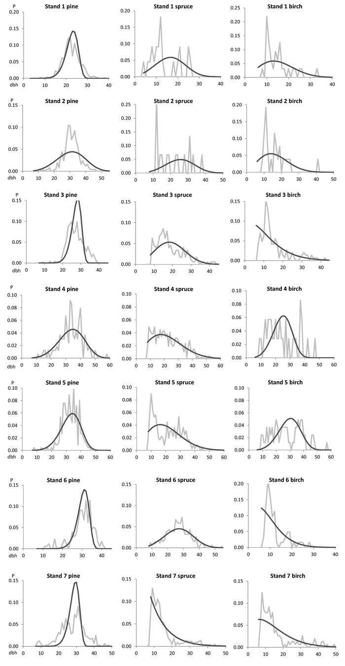
Fig. 1. The observed (grey line) and predicted (black line) species-specific breast height diameter (dbh) distributions for the modelling data set of seven clear-cut stands.
The goodness-of-fit was tested between the model-based distribution and the harvested distribution using the Kolmogorov-Smirnov (KS) goodness-of-fit test. KS test results were generally good. In only two out of 21 distributions, namely, stand no. 1 and 3, the distribution for pine rejected the KS test (Table 4).
| Table 4. Parameters b and c for the optimized Weibull distribution and the Kolmogorov-Smirnov (KS) goodness-of-fit statistics, i.e., supremum S, critical KS test value and KS-quotient by Tham (1988), for each distribution in the modelling data set. The restricted distributions (KS-q > 1.0) at the 0.1 significance level are shown in bold. | ||||||
| Stand | Species | b | c | S | KS test | KS-q |
| 1 | Pine | 27.65652 | 10.75086 | 0.0744 | 0.0516 | 1.4229 |
| Spruce | 22.84091 | 3.42576 | 0.1337 | 0.2609 | 0.5065 | |
| Birch | 17.08886 | 2.04147 | 0.1625 | 0.2164 | 0.7519 | |
| 2 | Pine | 33.85908 | 3.93423 | 0.0611 | 0.0774 | 0.7885 |
| Spruce | 28.18846 | 3.58795 | 0.2532 | 0.3160 | 0.7931 | |
| Birch | 18.15757 | 2.07353 | 0.1396 | 0.2400 | 0.5927 | |
| 3 | Pine | 28.54391 | 11.99995 | 0.0945 | 0.0562 | 1.5388 |
| Spruce | 21.48926 | 2.72832 | 0.0361 | 0.0925 | 0.4363 | |
| Birch | 14.6169 | 1.48271 | 0.0908 | 0.1020 | 0.8490 | |
| 4 | Pine | 36.92752 | 4.46618 | 0.0467 | 0.0956 | 0.4740 |
| Spruce | 24.96678 | 1.98449 | 0.0213 | 0.0566 | 0.8099 | |
| Birch | 28.00898 | 4.50419 | 0.0729 | 0.2069 | 0.3601 | |
| 5 | Pine | 35.85537 | 3.9325 | 0.0570 | 0.0818 | 0.5271 |
| Spruce | 25.53413 | 2.2826 | 0.0643 | 0.0648 | 0.8973 | |
| Birch | 32.39969 | 4.36577 | 0.0510 | 0.1352 | 0.8471 | |
| 6 | Pine | 32.92287 | 4.46401 | 0.0658 | 0.0923 | 0.7783 |
| Spruce | 29.96348 | 3.48296 | 0.0280 | 0.0658 | 0.3697 | |
| Birch | 9.88933 | 1.44835 | 0.1242 | 0.1554 | 0.7981 | |
| 7 | Pine | 29.8171 | 11.9427 | 0.0941 | 0.0686 | 0.9683 |
| Spruce | 13.22079 | 1.29523 | 0.0527 | 0.0574 | 0.6641 | |
| Birch | 17.06155 | 1.52872 | 0.0691 | 0.0989 | 0.6441 | |
3.2 Testing the application with practical timber trade contracts
The timber trade data set was used to test the optimization solution when the presented method was applied for practical data of clear-cut sections. The optimization found a converged distribution for all input characteristics. The average number of iterations needed for the solution was 24. First, we analysed how well the optimized distribution could provide the given input assortment volumes. The accuracy in the assortment volume estimates were very much influenced by the saw log reduction. If no reduction was assumed, then the difference between the input and output was 30 m3 (41%) in pulpwood volume and 1.53 m3 (1.3%) in saw log volume (Table 5). The average best fit was found using MELA05 saw log reduction. However, the relative difference in the pulpwood volume was still 6%, while that of log wood was only 0.4% (Table 5). The pulpwood characteristics were the most inaccurate for spruce, showing a 43 m3 (47%) underestimation (Table 5). Simultaneously, for pine, the underestimation in pulpwood was 40 m3 (45%) and for birch 6.7 m3 (16%) without saw log reduction. Using MELA05 reduction, these underestimations were 7.9, 1.2 and 4.4 m3 (8.6%, 1.4% and 10%) for spruce, pine and birch, respectively (Table 5). The saw log fraction could be considered to be accurate for each species and with and without saw log reduction (Table 5).
| Table 5. The difference (m3 for the clear-cut section) between the input assortment volumes from timber trade contracts and that of the output from the solved truncated Weibull distribution by tree species without saw log reduction and with the optional saw log reductions: MELA96, MELA05 and Bucking simulator (Malinen et al. 2007). The best results are shown in bold. | ||||||||
| Reduction: | Without | MELA96 | MELA05 | Bucking simulator | ||||
| Assortment: | Pulpwood | Saw logs | Pulpwood | Saw logs | Pulpwood | Saw logs | Pulpwood | Saw logs |
| Pine | 40.11 | 2.6 | 10.85 | 1.19 | 1.2 | 0.12 | 10.14 | 1.15 |
| Spruce | 43.49 | 2.27 | 39.96 | 2.16 | 7.86 | 0.63 | 32.26 | 1.81 |
| Birch | 6.65 | 0.32 | 4.39 | 0.58 | 4.39 | 0.54 | 3.46 | 0.53 |
| Total | 30.27 | 1.53 | 18.51 | 1.31 | 4.48 | 0.43 | 14.78 | 1.11 |
However, there were large differences in the volume characteristics between timber trade data and the real harvested data (Table 2). In the timber trade data, the total pulpwood was 10% underestimated, the log wood volume was 9% overestimated, and the harvested total stem number was 42% underestimated (Table 2). Second, we compared the optimized distributions to the harvested distribution.
More than half of the optimized distributions rejected the KS test (KS-q > 1.0) against the harvested distributions, namely, 69 cases without saw log reduction and 65–67 cases when the reductions were used out of 121 cases (Table 6). The average KS-q was largely the same with or without optional saw log reductions, namely, 1.379–1.423 versus 1.390 (Table 6). The best average error index (EI) values were found with the same option as the best KS test results (Table 6). The best species-specific fit was found without saw log reduction for pine, using an 18% MELA05 reduction for spruce and a 41% “Bucking simulator reduction” for birch. Thus, for spruce and birch, the highest applied reduction percentages provided the best fit between the modelled and harvested dbh distributions. The distributions for pine fitted clearly better than those for spruce or birch. This was mainly due to high number of understorey, small dimension pulpwood stems, which were common for birch and spruce admixtures. Indeed, about 60% of the distributions for spruce admixtures and 70% for birch admixtures resembled decreasing or strongly right-skewed distribution. At best, 12 distributions out of 41 distributions (29%) for pine rejected the KS test, when no saw log reduction was used.
| Table 6. The average goodness-of-fit tests according to the Kolmogorov-Smirnov quotient (KS-q) by Tham (1988) and the Error Index (EI) by Reynolds et al. (1988). Tests are given by tree species and total with the given saw log reduction option. The number of rejected cases (KS-q > 1) by tree species with the used saw log reduction percentage (slr%) in addition to the total number of rejected cases. The best results are shown in bold. | ||||||||
| Reduction | Without | MELA96 | MELA05 | Bucking simulator | ||||
| Test | KS-q | EI | KS-q | EI | KS-q | EI | KS-q | EI |
| Pine | 1.0755 | 0.5567 | 1.2637 | 0.6794 | 1.3584 | 0.7126 | 1.2687 | 0.6756 |
| Spruce | 1.5596 | 0.8457 | 1.5628 | 0.8344 | 1.3334 | 0.7500 | 1.5415 | 0.8287 |
| Birch | 1.5626 | 0.9844 | 1.4631 | 0.9062 | 1.4614 | 0.9080 | 1.4207 | 0.8771 |
| Total | 1.3903 | 0.7914 | 1.4226 | 0.8040 | 1.3787 | 0.7880 | 1.4034 | 0.7912 |
| KS test: | rejected | (slr%) | rejected | (slr%) | rejected | (slr%) | rejected | (sl%) |
| Pine | 12/41 | (0) | 18/41 | (16) | 20/41 | (24) | 19/41 | (18) |
| Spruce | 28/40 | (0) | 28/40 | (2) | 24/40 | (18) | 29/40 | (6) |
| Birch | 29/40 | (0) | 21/40 | (30) | 21/40 | (29) | 19/40 | (41) |
| Total | 69/121 | 67/121 | 65/121 | 67/121 | ||||
We noticed that the error in the estimated number of trees (calculated as the merchantable volume/average merchantable stem size) correlated most strongly with the lack-of-fit of the KS statistics. The correlation coefficient (r) was 0.45–0.49 for pine, 0.74–0.75 for spruce and 0.88–0.99 for birch. The higher correlation was always found for the solution when saw log reduction was used. Practically, the better the estimated number of harvested trees, the better the distribution fit (compatibility). There were practically no correlations between the KS statistics and the error in the saw log volume for pine (r 0.01) and the non-significant correlation for spruce and birch (r 0.06–0.26). The error in the pulpwood was negatively but non-significantly correlated with KS statistics (r from –0.08 to –0.23).
Typically, the saw log reduction resulted in a slightly weakened goodness-of-fit against the actual dbh distributions for pine. This result was because the distributions fitted considerably well without saw log reduction. Saw log reduction shifted the distribution toward larger dimensions, resulting in increasing lack-of-fit. One such example is shown in Fig. 2. In this case, the distribution without saw log reduction passed the KS test, but the distribution predicted with a 16% reduction barely rejected KS test (KS-q 1.07), and the last one which had a 24% reduction, was clearly rejected by the KS test (KS-q 1.76). In this example, the derived number of cut pines according to the timber trade was 1020, and the number of actual harvested pines was 930. On the other hand, Norway spruce usually benefited from the saw log reduction in terms of goodness-of-fit against the actual dbh distributions in our timber trade data set. At best, the improvement using an 18% saw log reduction for spruce was evident, as shown in Fig. 3. In this example, the derived number of cut spruces according to the timber trade was 704, and the number of harvested spruces was 1102. Fig. 4 represents an example for birch, which also benefited from a high saw log reduction percentage. In this case, the timber trade-based number of birch (533) was an overestimation, while the harvested number of birches was 207.
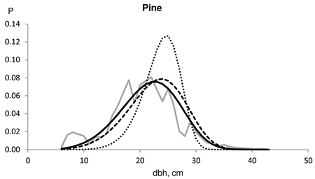
Fig. 2. Example of the harvested dbh distributions for Scots pine in test data (solid grey line). The number of harvested trees (N) and assortment volumes for a clear-cut section of 2.3 ha for the contract/harvester data were: N 1020/930; pulpwood 130/65 m3; saw logs 280/234 m3. The Kolmogorov-Smirnov quotient for the predicted distribution was 0.7719 without saw log reduction (solid line), 1.0738 using 16% MELA96 reduction (broken line) and 1.7620 using 24% MELA05 reduction (dotted line).
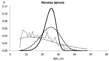
Fig. 3. Example of the harvested dbh distributions for Norway spruce in test data (solid grey line). The number of harvested trees (N) and assortment volumes for a clear-cut section of 2.7 ha for the contract/harvester data were: N 704/1102; pulpwood 100/74 m3; saw logs 255/302 m3. The Kolmogorov-Smirnov quotient for the predicted distribution was 2.608 without saw log reduction (solid line), 1.577 using 6% Bucking simulator-reduction (broken line) and 0.6777 with 18% MELA05 reduction (dotted line).
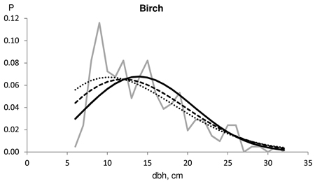
Fig. 4. Example of the harvested dbh distributions for birch in test data (solid grey line). The number of harvested trees (N) and the assortment volumes for a clear-cut section of 4.6 ha for the contract/harvester data were: N 533/207; pulpwood 70/30 m3; saw logs 10/2 m3. The Kolmogorov-Smirnov quotient for the predicted distribution was 0.766 without saw log reduction (solid line), 0.657 using 30% MELA96 reduction (broken line) and 0.600 with 41% Bucking simulator-reduction (dotted line).
4 Discussion
The objective of the study was to assess the accuracy of a theoretical diameter distribution optimized for pulpwood and saw log volumes. The diameter-height structure of a clear-cut stand was solved to generate tree dimensions for, among other things, the harvester’s bucking simulator. The need for the applied approach arose from the field. Indeed, forest companies need to know the structure of the stands marked for harvesting, to optimize the location and timing of the harvest operations, as well as the transportation and especially bucking, because in Finland, trees are cut to their final lengths already in the forest (Uusitalo 1997; Kivinen and Uusitalo 2002; Uusitalo et al. 2006; Malinen et al. 2007; Malinen et al. 2018). For a bucking simulator, the diameter-height distribution must be predicted, and the generated model-based tree dimensions and taper curves are then provided as input data. The actual minimum lengths and diameters for merchantable logs must be known to divide the growing stock into assortments (pulpwood and saw logs).
When we look at the presented modelling approach, we can say that the method itself performed well. In this method, the number of cut trees was, at first, estimated from the known input variables, including the pulpwood and saw log volume, as well as the average merchantable stem size of the cut trees. In the next step, after predicting the height curve, the parameters of the truncated Weibull distribution were optimized by minimizing the errors in the known assortment volumes. In this solution, the number of cut trees of merchantable dimensions was fixed, and the modelled tree heights did not vary during each species-specific optimization search for the optimal shape of the dbh distribution for a clear-cut stand. Similarly, Mehtätalo et al. (2007) treated the number of stems as a fixed value when they recovered the Weibull distribution from the total volume among other ALS-based stand characteristics.
To obtain successful optimization, we had to take care of the relevant starting values. The applied downhill simplex method (Nelder and Mead 1965) was shown to be somewhat sensitive to the starting guess. When the relevant starting values were sought, as they were here, looking for the best pair of integers b (8 ≤ b ≤ 45) and c (1 ≤ c ≤ 9.5) and using steps of size 0.1, the final solution was quite easily found, and it required typically less than 30 iterations. We also tried a widely distributed set of fixed starting points (b = 15, 20, 25 and c = 1.5, 3.5, 5.5), but the result was unsatisfactory. In this case, the solution was almost always symmetrical (c approximately 4), and thus, the solved distributions did not fit the typically skewed distributions for spruce and birch. According to Pukkala et al. (2010), the same simplex method worked well for the 3-parameter Weibull distribution, but they found difficulties with Johnson’s SB distribution, which had one more parameter to solve. In our study, the 2-parameter Weibull function was useful in reducing the number of decision variables (e.g., Bare and Opalach 1987). In certain instances, the 2-parameter Weibull distribution had performed even better than the 3-parameter Weibull function (Maltamo et al. 1995). The third parameter is typically for the minimum diameter. In this study, it was not needed because of the truncation according to the minimum pulpwood dimensions by tree species.
If the empirical distribution is bimodal, then the unimodal Weibull distribution is no longer the optimal option (e.g., the distribution for spruce in stand no. 5 in Fig. 1). Liu et al. (2002) represented a finite mixture model, which combined two Weibull distributions to achieve a bimodal structure. This method can offer an option if the assortment volumes are considerably erroneous when using only one unimodal Weibull distribution. However, the finite mixture model for two 2-parameter Weibull functions has five parameters to be solved, which might be a challenging task. Our optimization method held on to the original smooth form of the Weibull function from the truncation point on (Figs. 1, 2 and 3). The calibration estimation (Deville and Särndal 1992) does not stick out for a continuous smooth distribution. Instead, it can provide a two-mode or even multimodal distribution (creating peaks and/or hollows) as a solution when starting with the predicted Weibull distribution (Kangas and Maltamo 2000b; Kangas and Maltamo 2003). Even if the optimized Weibull distributions for pine had typically excess kurtosis, the generated pulpwood volume and especially the saw log volume were still accurate against the harvester data.
We need a prediction for the tree height to calculate the total and assortment volume for each tree. Näslund’s (1936) height curve has proved to be a good option among several two- or three-parameter height curves (see Mehtätalo et al. 2015). Among the validated stand characteristics, we found the highest bias in the mean height when using the models by Siipilehto and Kangas (2015). Thus, the height model might need calibration (Lappi 1991; Eerikäinen 2009). Siipilehto and Kangas (2015) showed that predicting the tree height was especially challenging when the input variables were assortment volumes instead of common stand characteristics, and therefore, they gave an example of calibrating the tree height using 1–5 measured sample trees. If it is possible to calibrate the height model during the harvest of the stand, the applied method can be still improved. For example, Uusitalo et al. (2006) tested an application for estimating the dbh distribution during harvest. The bias in tree height can be partly the result of the model for the missing tree tops in our STM data set. According to Varjo (1995), these models were reliable as long as the last cut diameter was below 10 cm. Holopainen et al. (2010) used successfully Varjo’s (1995) model. Siipilehto et al. (2016) noticed some especially large tree height estimates due to the last cut diameter being beyond 10 cm in the used harvester data. Optionally, total tree height (including stump) imputation for STM data could be done by fitting Laasasenaho’s (1982) taper curve (Räsänen et al. 1998; Malinen et al. 2014). Note that possible errors in stump height may also have an effect on tree height and on saw log recovery (see Korhonen et al. 2008).
The known assortment volumes were generated with satisfactory accuracy from the solved Weibull distribution, if the input variables were accurate. Thus, the presented method itself can be regarded as reliable. However, the reliability of the method in practice is highly dependent on the quality of the information available from the stand prior to clear-cutting.
The case study with the practical data of timber trade contracts showed that the converged solution for the Weibull distribution parameters could be found even if the input data was not accurate. The solved distribution could produce the saw log volume of the timber trade quite accurately regardless of the applied saw log reduction percentage. Simultaneously, the accuracy in the pulpwood volume was unsatisfactory. However, the inaccuracy in the pulpwood volume was only partly due to its visually assessed value in timber trade contracts. As can be seen in Table 3, the saw log and pulpwood volumes were both only slightly biased for pine and spruce (1–13%). The main reason for the inaccurate pulpwood volume was simply the overestimated average merchantable stem size, which in turn resulted in clear underestimation of the number of harvested trees (31–61%). The underestimation of the stem number made it impossible to generate the input assortment volumes. Thus, typically wide and skewed distributions for spruce and birch were given a bell-shaped distribution, which resulted in a significant lack-of-fit. We determined that the error in the estimated stem number was highly correlated with the lack-of-fit, i.e., with the KS statistics or error index (EI). When saw log reduction was used, the combination of assortment volume and number of cut trees became more relevant. Indeed, the optimized Weibull distribution was able to provide the input assortments much more precisely using saw log reduction. Finally, the compatibility between the timber trade input and model output was better the higher the saw log reduction percentage was (Table 5). Unfortunately, this improvement for pine was not realized when the distributions were analysed toward the real harvested distributions (Table 6).
According to a case study with the practical data of timber trade contracts, the average merchantable stem size was shown to be a bottleneck for successful fitting. The reason for difficulties was connected to decreasing or strongly right-skewed dbh distributions, which were common for spruce and birch in the data set used for validation. When the estimate for the harvested stem number is a clear underestimation, the sampled trees must be large enough to achieve the given assortment volumes. This circumstance, in turn, resulted in peaked distributions that included large trees. Thus, the typical decreasing or highly skewed distributions for spruce and birch were not provided by the model due to a 40–60% underestimation in the stem number. Finally, 24–29 distributions for spruce and 19–29 for birch out of 40 cases rejected the KS test. At best, when saw log reduction was not used for pine, 12 distributions (29%) out of 41 rejected the KS test. In our case, the goodness-of-fit tests using KS or EI showed compatible results. However, this finding is not necessarily always the situation. Indeed, Siipilehto et al. (2016) found differences between applied methods when ranking them according to alternative goodness-of-fit statistics. For this reason, it is recommended to apply several goodness-of-fit statistics (Reynolds et al. 1988; Cao 2004).
In conclusion, the results of the presented method were twofold. On the one hand, the method could provide the assortment volumes accurately while satisfying the goodness-of-fit to the harvested dbh distributions. On the other hand, the practical timber trade data showed such underestimation in the number of cut trees that the presented method could not provide satisfactory dbh distributions. Similar to the results with timber trade data, the recent studies of the optional pre-harvest inventory methods (e.g. SWFI, alternative ALS-based methods, Trestima) for clear-cutting stands have shown considerable inaccuracy in species-specific volume characteristics or lack-of-fit in dbh distributions (Korhonen et al. 2008; Holopainen et al. 2010; Siipilehto et al. 2016). Overall, the quality of the data is important for optimal decision making (Eid et al. 2004; Duvemo and Lämås 2006; Mäkinen et al. 2010; Mäkinen et al. 2012). As Holopainen et al. (2010) stated, operative pre-harvest measurements would require more accurate input data than the current methods. Additional field measurements (e.g., EMO method) help to capture the shape of the dbh distributions, especially the largest pines (see Siipilehto et al. 2016). We believe that the estimation of timber trade variables could be helped, if the input assortment volumes and the average stem size have been converted to the harvestable number of stems already in the field. Or vice versa, it is possible to estimate the number of cut trees in the field, which is then converted to the average stem size required by the contract. Theoretically, the presented method can be used abroad as well, whenever the input data consists of pre-harvest assortment volumes and the average stem size and the minimum assortment diameters for bucking are known. Note that if the average stem size is not available, the presented method does not work. For such cases, we must determine other approaches, e.g., compose prediction models for the number of commercial stems from the assortment volumes or iteratively search for the optimal number of cut trees. Also, the additional ALS based inventory data could be useful e.g., when predicting the number of stems and the diameter-height relationship.
Acknowledgements
We would like to thank Juha Lappi for the valuable help concerning optimization. We also thank the anonymous reviewers for their comments on the manuscript. This study was conducted in Natural Resources Institute Finland (Luke).
References
Arlinger J., Möller J.J., Sorsa J.-A., Räsänen T. (2012). Introduction to StanForD2010. Structural descriptions and implementation recommendations. Skogforsk. 74 p.
Bailey R.L., Dell T.R. (1973). Quantifying diameter distributions with the Weibull function. Forest Science 19: 97–104.
Bare B.B., Opalach D. (1987). Optimizing species composition in uneven-aged forest stands. Forest Science 33: 958–970.
Borders B.E., Souter R.A., Bailey R.L., Ware K.D. (1987). Percentile-based distributions characterize forest stand tables. Forest Science 33: 570–576.
Cajander A.K. (1926). The theory of forest types. Acta Forestalia Fennica 29(3). 108 p. https://doi.org/10.14214/aff.7193.
Cao Q.V. (2004). Predicting parameters of a Weibull function for modeling diameter distribution. Forest Science 50: 682–685.
Deville J.C., Särndal C.E. (1992). Calibration estimators in survey sampling. Journal of American Statistical Association 87(418): 376–382. https://doi.org/10.1080/01621459.1992.10475217.
Duvemo K., Lämås T. (2006). The influence of forest data quality on planning processes in forestry. Scandinavian Journal of Forest Research 21(4): 327−339. https://doi.org/10.1080/02827580600761645.
Eerikäinen K. (2009). A multivariate linear mixed-effects model for the generalization of sample tree heights and crown ratios in the Finnish National Forest Inventory. Forest Science 55: 480–493.
Eid T., Gobakken T., Næsset E. (2004). Comparing stand inventories for large areas based on photo-interpretation and laser scanning by means of cost-plus-loss analyses. Scandinavian Journal of Forest Research 19(6): 512−523. https://doi.org/10.1080/02827580410019463.
Holopainen M., Vastaranta M., Rasinmäki J., Kalliovirta J., Mäkinen A., Haapanen R., Melkas T., Yu X., Hyyppä J. (2010). Uncertainty in timber assortment estimates predicted from forest inventory data. European Journal of Forest Research 129(6): 1131–1142. https://doi.org/10.1007/s10342-010-0401-4.
Holopainen M., Vastaranta M., Hyyppä J. (2014). Outlook for the next generation’s precision forestry in Finland. Forests 5(7): 1682–1694. https://doi.org/10.3390/f5071682.
Hyink D.M., Moser J.W. (1983). A generalized framework for projecting forest yield and stand structure using diameter distributions. Forest Science 29: 85–95.
Kangas A., Maltamo M. (2000a). Percentile based basal area diameter distribution models for Scots pine, Norway spruce and birch species. Silva Fennica 34(4): 371–380. https://doi.org/10.14214/sf.619.
Kangas A., Maltamo M. (2000b). Calibrating predicted diameter distribution with additional information. Forest Science 46: 390–396.
Kangas A., Maltamo M. (2003). Calibrating predicted diameter distribution with additional information in growth and yield predictions. Canadian Journal of Forest Research 33(3): 430–434. https://doi.org/10.1139/x02-121.
Kangas A., Heikkinen E., Maltamo M. (2004). Accuracy of partially visually assessed stand characteristics: a case study of Finnish forest inventory by compartments. Canadian Journal of Forest Research 34(4): 916–930. https://doi.org/10.1139/x03-266.
Kivinen V.-P., Uusitalo J. (2002). Applying fuzzy logic to tree bucking control. Forest Science 48: 673–684.
Korhonen L., Peuhkurinen J., Malinen J., Suvanto A., Maltamo M., Packalén P., Kangas J. (2008). The use of airborne laser scanning to estimate sawlog volumes. Forestry 81(4): 499–510. https://doi.org/10.1093/forestry/cpn018.
Laasasenaho J. (1982). Taper curve and volume functions for pine, spruce and birch. Communicationes Instituti Forestalis Fenniae 108. 74 p. http://urn.fi/URN:ISBN:951-40-0589-9.
Laasasenaho J., Päivinen R. (1986). Kuvioittaisen arvioinnin tarkastamisesta. [On the checking of inventory by compartments]. Folia Forestalia 664. 19 p. http://urn.fi/URN:ISBN:951-40-0757-3.
Lappi J. (1991). Calibration of height and volume equations with random parameters. Forest Science 37: 781−801.
Lappi J. (1997). A longitudinal analysis of height/diameter curves. Forest Science 43: 555–570.
Liu C., Zhang L., Davis C.J., Solomon D.S., Gove J.H. (2002). A finite mixture model for characterizing the diameter distributions of mixed-species forest stands. Forest Science 48: 653–661.
Mäkinen A., Kangas A., Mehtätalo L. (2010). Correlations, distributions, and trends in forest inventory errors and their effects on forest planning. Canadian Journal of Forest Research 40(7): 1386–1396. https://doi.org/10.1139/X10-057.
Mäkinen A., Kangas A., Nurmi M. (2012). Using cost-plus-loss analysis to define optimal forest inventory interval and forest inventory accuracy. Silva Fennica 46(2): 211–226. https://doi.org/10.14214/sf.55.
Malinen J., Kilpeläinen H., Piira T., Redsven V., Wall T., Nuutinen T. (2007). Comparing model-based approaches with bucking simulation-based approach in the prediction of timber assortment recovery. Forestry 80(3): 309–321. https://doi.org/10.1093/forestry/cpm012.
Malinen J., Kilpeläinen H., Ylisirniö K. (2014). Description and evaluation of Prehas software for pre-harvest assessment of timber assortments. International Journal of Forest Engineering 25(1): 66–74. https://doi.org/10.1080/14942119.2014.902686.
Maltamo M. (1997). Comparing basal area diameter distributions estimated by tree species and for the entire growing stock in a mixed stand. Silva Fennica 31(1): 53–65. https://doi.org/10.14214/sf.a8510.
Maltamo M., Kangas A. (1998). Methods based on k-nearest neighbor regression in the prediction of basal area diameter distribution. Canadian Journal of Forest Research 28(8): 1107–1115. https://doi.org/10.1139/x98-085.
Maltamo M., Puumalainen J., Päivinen R. (1995). Comparison of beta and Weibull functions for modelling basal area diameter distribution in stands of Pinus sylvestris and Picea abies. Scandinavian Journal of Forest Research 10(1–4): 284–295. https://doi.org/10.1080/02827589509382895.
Mehtätalo L. (2002). Valtakunnalliset puukohtaiset tukkivähennysmallit männylle, kuuselle, koivulle ja haavalle. [Log reduction models for the stems of pine, spruce birches and aspen in Finland]. Metsätieteen aikakauskirja 4/2002: 575–591. https://doi.org/10.14214/ma.6196.
Mehtätalo L. (2004). A longitudinal height-diameter model for Norway spruce in Finland. Canadian Journal of Forest Research 34(1): 131–140. https://doi.org/10.1139/x03-207.
Mehtätalo L. (2005). Height-Diameter (H-D) models for Scots pine and birch in Finland. Silva Fennica 39(1): 55–66. https://doi.org/10.14214/sf.395.
Mehtätalo L., Maltamo M., Packalén P. (2007). Recovering plot-specific diameter distribution and height-diameter curve using ALS based stand characteristics. ISPRS Workshop on Laser Scanning 2007 and SilviLaser 2007, Espoo, September 12–14, Finland.
Mehtätalo L., De-Miguel S., Gregoire T.G. (2015). Modeling height-diameter curves for prediction. Canadian Journal of Forest Research 45(7): 826–837. https://doi.org/10.1139/cjfr-2015-0054.
Merganič J., Sterba H. (2006). Characterisation of diameter distribution using the Weibull function: method of moments. European Journal of Forest Research 125(4): 427–439. https://doi.org/10.1007/s10342-006-0138-2.
Mouer M., Stage A.R. (1995). Most similar neigbor: an improved sampling inference procedure for natural resource planning. Forest Science 41: 337–359.
Näslund M. (1936). Skogsförsöksanstaltens gallringsförsök i tallskog. [Forest research institute’s thinning experiment for pine]. Meddelanden från Statens Skogsförsöksanstalt 29. 169 p.
Nelder J.A., Mead R. (1965). A simplex method for function minimization. Computer Journal 7(4): 308–313. https://doi.org/10.1093/comjnl/7.4.308.
Packalén P. , Maltamo M. (2008). Estimation of species-specific diameter distributions using airborne laser scanning and aerial photographs. Canadian Journal of Forest Research 38(7): 1750–1760. https://doi.org/10.1139/X08-037.
Palahi M., Pukkala T., Blasco E., Trasobares A. (2007). Comparison of Johnson’s SB, Weibull and truncated Weibull functions for modelling the diameter distribution of forest stands in Catalonia (north-east of Spain). European Journal of Forest Research 126(4): 563–571. https://doi.org/10.1007/s10342-007-0177-3.
Petterson H. (1995). Barrskogens volymproduction. [Volume production for conifer forests]. Meddelanden från Statens Skogforkningsinstitut 45. 399 p.
Peuhkurinen J., Maltamo M., Malinen J. (2007). Preharvest measurement of marked stands using airborne laser scanning. Forest Science 53: 653–661.
Peuhkurinen J., Maltamo M., Malinen J. (2008). Estimating species-specific diameter distributions and saw log recoveries of boreal forests from airborne laser scanning data and aerial photographs: a distribution-based approach. Silva Fennica 42(4): 625–641. https://doi.org/10.14214/sf.237.
Peuhkurinen J., Mehtätalo L., Maltamo M. (2011). Comparing individual tree detection and the area-based statistical approach for retrieval of forest stand characteristics using airborne laser scanning in Scots pine stands. Canadian Journal of Forest Research 41(3): 583–598. https://doi.org/10.1139/X10-223.
Poso S. (1983). Kuvioittaisen arvioimismenetelmän perusteita. [Basic features of inventory by compartments]. Silva Fennica 17(4): 313–349. https://doi.org/10.14214/sf.a15179.
Press W.H., Teukolsky S.A., Vetterling W.T., Flannery B.P. (1992). Numerical recipes in FORTRAN: the art of scientific. 2nd ed. Cambridge University Press. 963 p.
Pukkala T., Lähde E., Laiho O. (2010). Optimizing the structure and management of uneven-sized stands of Finland. Forestry 83(2): 129–142. https://doi.org/10.1093/forestry/cpp037.
Räsänen T., Aaltonen A., Lindroos J., Lukkarinen E., Vuorenpää T. (1998). Puustotiedon hankinta hakkuukoneella. [Harvester data collection]. Metsätehon raportti 44. 32 p.
Redsven V., Anola-Pukkila A. Haara A., Hirvelä H., Härkönen K., Kettunen L., Kiiskinen A., Kärkkäinen L., Lempinen R., Muinonen E., Nuutinen T., Salminen O., Siitonen M. (2005). MELA2005 reference manual. Finnish Forest Researh Institute. 621 p. http://www.metla.fi/metinfo/mela/tuotteet/mela2005.pdf.
Reynolds M.R., Burk T.E., Huang W.C. (1988). Goodness-of-fit tests and model selection procedures for diameter distribution models. Forest Science 34: 373–399.
Siipilehto J. (1999). Improving the accuracy of predicted basal-area diameter distribution in advanced stands by determining stem number. Silva Fennica 33(4): 281–301. https://doi.org/10.14214/sf.650.
Siipilehto J., Mehtätalo L. (2013). Parameter recovery vs. parameter prediction for the Weibull distribution validated for Scots pine stands in Finland. Silva Fennica 47(4) article 1057. https://doi.org/10.14214/sf.1057.
Siipilehto J., Kangas A. (2015). Näslundin pituuskäyrä ja siihen perustuvia malleja läpimitta-pituus riippuvuudesta suomalaisissa talousmetsissä. [Näslund’s hight curve models for the diameter-height relationship in Finnish commercial forests]. Metsätieteen aikakauskirja 4/2015: 215–236. https://doi.org/10.14214/ma.6584.
Siipilehto J., Lindeman H., Vastaranta M., Yu X., Uusitalo J. (2016). Reliability of the predicted stand structure for clear-cut stands using optional methods: airborne laser scanning-based methods, smartphone-based forest inventory application Trestima and pre-harvest measurement tool EMO. Silva Fennica 50(3) article 1568. https://doi.org/10.14214/sf.1568.
Siitonen M., Härkönen K., Hirvelä H., Jämsä J., Kilpeläinen H., Salminen O., Teuri M. (1996). MELA Handbook 1996 Edition. The Finnish Forest Research Institute, Research Paper 622. 452 p. http://urn.fi/URN:ISBN:951-40-1543-6.
Tham Å. (1988). Structure of Mixed Picea abies (L.) Karst. and Betula pendula Roth and Betula pubescens Ehrh. stands in South and Middle Sweden. Scandinavian Journal of Forest Research 3(1–4): 355–369. https://doi.org/10.1080/02827588809382523.
Uusitalo J. (1997). Pre-harvest measurement of pine stands for sawing production planning. Acta Forestalia Fennica 259. 56 p. https://doi.org/10.14214/aff.7519.
Uusitalo J., Puustelli A., Kivinen V.-P., Nummi T., Sinha B.K. (2006). Bayesian estimation of diameter distribution during harvesting. Silva Fennica 40(4): 663–671. https://doi.org/10.14214/sf.321.
Varjo J. (1995). Latvan hukkaosan pituusmallit männylle, kuuselle ja koivulle metsurimittausta varten. [The height model for the waste top section of the stem for pine, spruce and birch]. In: Verkasalo E. (ed.). Puutavaran mittauksen kehittämistutkimuksia 1989–93. Metsäntutkimuksen tiedonantoja 558: 21–23. http://urn.fi/URN:ISBN:951-40-1434-0.
Vauhkonen J., Packalen P., Malinen J., Pitkänen J., Maltamo M. (2014). Airborne laser scanning-based decision support for wood procurement planning. Scandinavian Journal of Forest Research 29(sup1): 132–143. https://doi.org/10.1080/02827581.2013.813063.
Total of 62 references.
