Olga Grigorieva,
Olga Brovkina  ,
Alisher Saidov
,
Alisher Saidov
An original method for tree species classification using multitemporal multispectral and hyperspectral satellite data
Grigorieva O., Brovkina O., Saidov A. (2020). An original method for tree species classification using multitemporal multispectral and hyperspectral satellite data. Silva Fennica vol. 54 no. 2 article id 10143. https://doi.org/10.14214/sf.10143
Highlights
- Differences between spectral reflectance of tree species are statistically significant in the sub-seasons of spring, first half of summer, and main autumn
- Classification using multitemporal multispectral data is more productive than is classification using a single hyperspectral image
- the method improves recent forest mapping in the study regions.
Abstract
This study proposes an original method for tree species classification by satellite remote sensing. The method uses multitemporal multispectral (Landsat OLI) and hyperspectral (Resurs-P) data acquired from determined vegetation periods. The method is based on an original database of spectral features taking into account seasonal variations of tree species spectra. Changes in the spectral signatures of forest classes are analyzed and new spectral–temporal features are created for the classification. Study sites are located in the Czech Republic and northwest (NW) Russia. The differences in spectral reflectance between tree species are shown as statistically significant in the sub-seasons of spring, first half of summer, and main autumn for both study sites. Most of the errors are related to the classification of deciduous species and misclassification of birch as pine (NW Russia site), pine as mixture of pine and spruce, and pine as mixture of spruce and beech (Czech site). Forest species are mapped with accuracy as high as 80% (NW Russia site) and 81% (Czech site). The classification using multitemporal multispectral data has a kappa coefficient 1.7 times higher than does that of classification using a single multispectral image and 1.3 times greater than that of the classification using single hyperspectral images. Potentially, classification accuracy can be improved by the method when applying multitemporal satellite hyperspectral data, such as in using new, near-future products EnMap and/or HyspIRI with high revisit time.
Keywords
boreal forest;
phenological period;
space spectroscopy;
spectral signature
- Grigorieva, A.F. Mozhaysky’s Military-Space Academy, Krasnogo Kursanta Street 19a, 197198, Saint Petersburg, Russia E-mail alenka12003@gmail.com
-
Brovkina,
Global Change Research Institute CAS, Bělidla 986/4a, 603 00, Brno, Czech Republic
E-mail
brovkina.o@czechglobe.cz
- Saidov, A.F. Mozhaysky’s Military-Space Academy, Krasnogo Kursanta Street 19a, 197198, Saint Petersburg, Russia E-mail celestial.azura@gmail.com
Received 22 January 2019 Accepted 18 February 2020 Published 2 March 2020
Views 82157
Available at https://doi.org/10.14214/sf.10143 | Download PDF

1 Introduction
Monitoring of forests is one of the relevant and practical tasks effectively carried out on the basis of recent satellite optical–electronic multispectral (MS) and hyperspectral (HS) means (Boyd et al. 2005; Banskota et al. 2014; Transon et al. 2017). MS and HS data referencing spectra of woody vegetation and algorithms of data processing in (semi)automatic mode allow separation of forest from non-forest lands (Connette et al. 2016; Zhou et al. 2018); prediction of forest inventory characteristics (McRoberts et al. 2007); and detection of forest damage due to fires, degradation, and pathological changes (Grigorieva 2014; Lausch et al. 2016; Brovkina et al. 2017).
Among the tasks related to forest monitoring, classification of forests by tree species composition is one of the most complex. That is because the spectral properties of different forest formations can vary significantly depending on the vegetation period, crown closure, growth, and conditions under which the data were acquired. The spectral variability within species may be even greater than is the variability between species (Grigorieva et al. 2012). Only few tree species can be distinguished with satisfactory classification accuracy based upon satellite data from a single vegetation period. Pax-Lenney et al. (2001) evaluated the ability of a neural network to identify coniferous forests using a Landsat thematic mapper (TM) midsummer data set and determined mean classification accuracy within a region of around 85%. Using maximum likelihood classifier, Shataee et al. (2004) showed a classification accuracy of 61% in identifying six forest types based on Landsat enhanced thematic mapper (ETM) data. Galidaki and Gitas (2014) investigated the potential of using Hyperion imagery and a nearest neighbor classifier to map four forest species. Their classification accuracy ranged from 72% to 83%.
Significant errors are observed in particular when processing a single satellite scene, because within one season, as a rule, it is impossible to reliably classify the entire diversity of the species composition for species having close spectral features in several spectral bands (Hovi et al. 2017). Shafri et al. (2007) found that classification of mixed forests into four tree species classes achieved accuracy ranging from 49% using a spectral angle mapper to 86% using an artificial neural network based on a single hyperspectral image. Immitzer et al. (2016) used an MS satellite Sentinel-2 scene with supervised random forest classifier to map seven different deciduous and coniferous tree species with a cross-validated overall accuracy of 65%. Waser et al. (2014) achieved a promising classification accuracy of 83% using high spatial resolution down to 2 m in a MS WorldView-2 single summer scene to classify seven tree species.
Increased effectiveness in tree species classification can be achieved by processing satellite MS or HS data acquired in different phenological periods. Even using two satellite scenes from different phenological periods can provide significantly better classification results compared to processing a single satellite scene (Hill et al. 2010). Tigges et al. (2013) used a time series of RapidEye data including five dates to classify eight tree genera. The best classification they achieved was estimated at accuracy of 83%. Sheeren et al. (2016) used Formosat-2 images acquired on 17 dates to classify 13 tree species with classification accuracies of 90–93%. Some studies have used seasonal statistics of vegetation indices and textural features as indicators of tree species (Sasaki et al. 2001; Arekhi et al. 2017). Seasonal variation of widespread biophysical indices coincide for some boreal tree species, however, and so their use is not effective (Grigorieva et al. 2017).
In the context of the studies cited above identifying tree species, the use of informative spectral bands of MS and HS data seems promising in the optimal seasons of the year, when the spectral difference of each tree species is at its maximum. The main objective of this study was to develop and implement a method for identifying tree species from MS and HS satellite data using 1) a series of multitemporal satellite data acquired in determined phenological periods of tree species, and 2) a system of various spectral–temporal features of tree species. A specific objective was to compare the proposed method from multitemporal satellite data with existing methods of tree species classification from single MS and single HS images.
2 Materials and methods
2.1 Study area
Study areas are located in the northeastern part of the Gulf of Finland (Baltic Sea) within the Leningrad Region, Russia (Berezovye Islands archipelago, 60°23´N, 28°26´E) and in the eastern Moravian–Silesian Region, Czech Republic (Těšínské Beskydy Mountains, 49°37´N, 18°47´E) (Fig. 1).
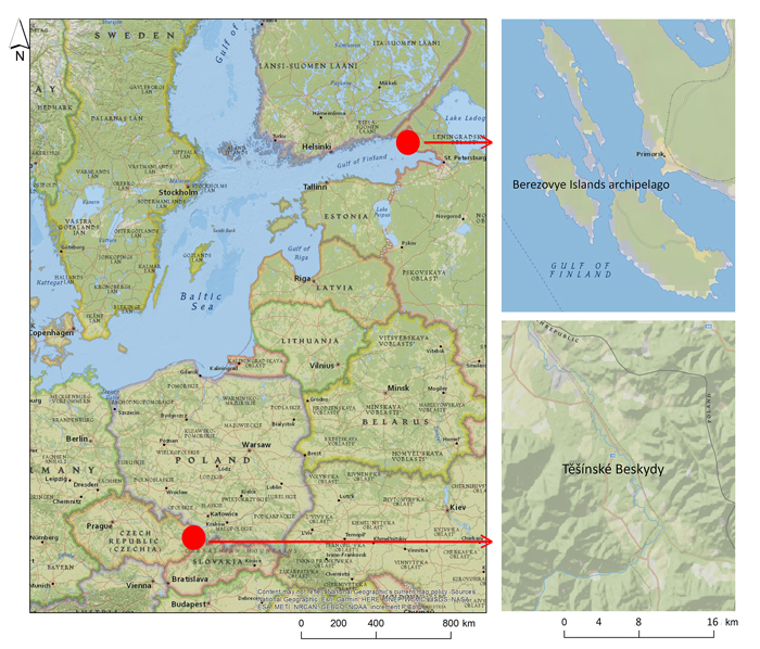
Fig. 1. Study areas: Berezovye Islands archipelago (Russia) and Těšínské Beskydy Mountains (Czech Republic).
The forest stands in the Berezovye Islands archipelago are composed of Scots pine (Pinus sylvestris L.) predominating in the poorest, swampy soils, as well as Norway spruce (Picea abies (L.) H. Karst.), European white birch (Betula pendula Roth), and grey alder (Alnus glutinosa (L.) Gaertn.) (Bohn et al. 2000; Stepanchikova et al. 2011). Pine and birch cover the main part of the islands. All of the forests have several times been harvested using logging machinery, and many have been exposed to surface fires and crown fires. The length of the vegetation season in the region is about 150–170 days (Leningrad region. Nature and Economy 1958).
The forest stands in the Těšínské Beskydy Mountains are mainly composed of managed Norway spruce (P. abies) and European beech (Fagus sylvatica L.) as the dominant tree species. There exists also a scattered mixture of Scots pine (P. sylvestris), silver fir (Abies alba Mill.), European larch (Larix decidua Mill.), and ash (Fraxinus excelsior L.) (Michalko 1986). The length of the vegetation season in the region is about 186–190 days (Hajkova et al. 2012).
2.2 Data
Multispectral Landsat-8 satellite OLI data (NASA, http://earthexplorer.usgs.gov.) and hyperspectral Resurs-P satellite data (RosCosmos, http://eng.ntsomz.ru.) were used in the study (Table 1). Radiometric correction was made to reduce or correct errors in the raw digital numbers in the images. The raw digital numbers were converted to top-of-atmosphere radiance by rescaling the data with sensor-specific information and removing the effects of differences in illumination geometry (different solar angle, Earth–Sun distance). Atmospheric correction was done to remove the effects of the atmosphere and to produce surface reflectance values. The atmospheric correction of Landsat images was done in the FLAASH module of ENVI 4.4 software. The atmospheric correction of Resurs-P images was performed in MODTRAN 5.2 software using meteorological observations on the acquisition date and place (60°23´N, 28°26´E) and the method by Brovkina et al. (2016).
| Table 1. Satellite multispectral (MS) and hyperspectral (HS) acquisition dates used in the study. | |||||||||
| Study area | Acquisition date in 2015 | ||||||||
| MS | HS | ||||||||
| Berezovye Islands | 11.04 | 6.05 | 13.05 | 14.06 | 30.06 | 15.08 | 31.08 | 11.10 | 30.05 |
| Těšínské Beskydy | 23.04 | 30.04 | 16.05 | 12.07 | 19.07 | 13.08 | 14.09 | 1.11 | 6.06 |
A geobotanical map of the Berezovye Islands (Volkova et al. 2016) provided the basis for construction of training samples as well as verification of the classification method. The map contained the main types of forest vegetation: coniferous, small-leaved, and broad-leaved forests. According to the prevalence of tree species, these types have been distinguished: spruce, pine, spruce–pine (as an independent unit), birch, aspen, and black alder. Based on the characteristics of grass–shrub and moss–lichen layers, five groups of associations were identified in the pine forests: green pine forests, bilberry pine, herbaceous pine, sphagnum pine, and pine forests of sandy beaches and dunes.
A forest inventory map provided by the Forest Management Institute (www.uhul.cz) was used in the Těšínské Beskydy study area (49°37´N, 18°47´E). Forest management planning data contained more than 30 characteristics for each forest compartment collected in compliance with the Czech forest management planning standard (Stanek et al. 1997). In this study, we used the information about the type of forest, tree species, share of tree species, and forest compartments.
2.3 Method for tree species classification from multitemporal satellite data
The proposed method for tree species classification based on multitemporal data consisted of two main stages (Fig. 2). At the first stage, image fragments (background) not related to the forest were excluded from the further processing based on an analysis of seasonal changes in the normalized difference vegetation index (NDVI). At the second stage, changes in the spectral signatures of forest classes were analyzed and new spectral–temporal features were created for the classification (Grigorieva et al. 2017).
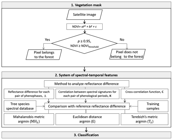
Fig. 2. Structure of the proposed method for tree species classification from multitemporal multispectral satellite data. F is a number of phenophase, a,b,c are approximation coefficients, NDVI is normalized difference vegetation index.
2.3.1 Vegetation mask
Phenological phases (or phenophases) of forest vegetation were used in the study. Phenological phase refers to a specific time period in the annual life cycle of trees that can be defined by a start and end point. Because the maximum NDVI values refer not only to forest vegetation in the active vegetation phenophase but also to other plant species, an additional feature was used to distinguish image pixel(s) with forest: the function NDVI = f(F) approximated by a quadratic function NDVI = aF2 + bF + c, where F is number of phenophase (paragraph 2.3.4). To obtain the phenophase corresponding to the date of acquired satellite images, the table data is interpolated:
F = 0.023DOY + 0.74 ,
where DOY is day of year. For example, for Berezovye Islands archipelago the end of phen_3 lie between 11.4 and 15.5, which is correspond to 102 and 129 DOY. The next satellite images were acquired for mentioned period: 11.04, 06.05 and 13.05 (105, 127 and 134 DOY). Using linear interpolation, F obtained for these images were: F = 3.15, F = 3.66 and F = 3.82.
The following rule was applied to decide whether an image pixel does or does not belong to forest: If seasonal variations of NDVI can be approximated by a quadratic function with a confidence value of p = 0.95 and its value in the most active phase of vegetation is greater than or equal to the NDVI threshold value, then the pixel belongs to the forest. For each species, the threshold was the lowest NDVI from all training samples. NDVI threshold value was calculated from the reference spectrum at the corresponding phenophase.
In the case of only two satellite images from two phenophases, the following rule is applied: If the correlation between the spectra of the two phenophases was high (k ≥ 0.97) and NDVI in the most active vegetation period was less than the NDVI threshold, then the pixel belongs to the background and it was excluded from further processing.
2.3.2 System of new spectral–temporal features for forest classes
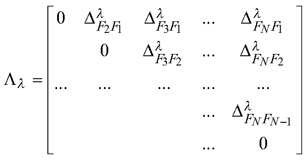
New spectral–temporal features created for the classification included a reflectance difference (Δ) for each pixel of each pair (i, j) of images from corresponding phenophases: ![]() where λ is a wavelength, and r is a reflectance value. As a result, M diagonal matrices Λλ of size N × N are obtained, where M is the number of spectral bands, and N is the number of images acquired in the corresponding phenophases:
where λ is a wavelength, and r is a reflectance value. As a result, M diagonal matrices Λλ of size N × N are obtained, where M is the number of spectral bands, and N is the number of images acquired in the corresponding phenophases:
M matrices are transformed into one matrix, Λ, of size ((N2 – N)/2) × M for further calculation of correlation ![]() between spectral signatures for each pair (i, j) of phenophase. The correlation characterizes how the reflectance depends on the phenophase. As a result, matrix K of size N × N is obtained:
between spectral signatures for each pair (i, j) of phenophase. The correlation characterizes how the reflectance depends on the phenophase. As a result, matrix K of size N × N is obtained:
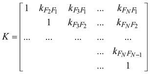
Matrix K is transformed into the vector of features K of size ((N2 – N)/2) × 1 for further calculations.
Coefficients of the cross-correlation function between reflectance at various phenological periods are calculated as:
where r(λ,F) is the reflectance function of two variables: wavelength λ = λ1,…,λM and phenological period F = F1,…,FN; r’(λ,F) = r(λ,F) – S[r(λ,F)] is the centered realization of point (λ,F) for function r(λ,F); S[r(λ,F)] is the mathematical expectation of the reflectance r(λ,F); σr(λ,F) is the mean square deviation of function r(λ,F); n is offset value relative to phenophase; and m is offset value relative to the spectral band.
As a result, a matrix С of size (2M − 1) × N2 is obtained that allows tracking reflectance changes from one vegetation phase to another and estimating these changes for various spectral bands:
2.3.3 Comparison of the reflectance difference obtained with reference reflectance difference
Depending on the classification method, three measures were used to compare the reflectance difference obtained (matrix C) with the reference reflectance difference: Mahalanobis metric (MHλ), Euclidian distance (E) (Schowengerdt 2006), and Terebizh’s metric (Tλ) (Terebizh 2005). The Euclidian distance is only effective in the case of small linear dimensions, and it was used to calculate the proximity measure of the reference value and pixel:

where ![]() and
and ![]() are elements of the matrix K for image and reference, respectively. Mahalanobis and Terebizh’s metrics were used to compare matrices Λ and C. These metrics were calculated for each spectral band as follows:
are elements of the matrix K for image and reference, respectively. Mahalanobis and Terebizh’s metrics were used to compare matrices Λ and C. These metrics were calculated for each spectral band as follows:
![]()
where ![]() and
and ![]() are columns of matrix Λ for image and reference, respectively; and
are columns of matrix Λ for image and reference, respectively; and ![]() is the covariance matrix of features
is the covariance matrix of features ![]() for reference. The class to which a pixel belongs was defined based on the highest frequency of occurrence of such event, Pk, where the selected measure took the minimum values:
for reference. The class to which a pixel belongs was defined based on the highest frequency of occurrence of such event, Pk, where the selected measure took the minimum values:
kλ = argmin(MHλ) and kλ = argmin(Tλ); Pk = nk /M; k = argmaxPk ,
where k – class number, kλ – class number for which the selected measure took the minimum values at the wavelength λ, nk – class number, for which the selected measure took the minimum values at all wavelengths.
2.3.4 Database of tree species spectral features
The method proposed in this study involves a specialized tree species spectral features database (DB) based on long-term ground-based and remote-sensing observations of phenology. Use of the DB can help to reduce temporal and regional variability in the spectra of forest vegetation caused by the diversity of natural conditions in different areas. Phenophases of main tree species were derived based on ground-based and remote-sensing observations of phenology for both study sites. For Těšínské Beskydy, the atlas of phenological conditions of the Czech Republic also was used (Hájková et al. 2012). The DB of reflectance spectra takes into account peculiarities of the beginning and end of phenophases of the main tree species across study areas (Grigorieva et al. 2012). The DB is integrated with a geographic information system, where a specially created terrain model with attribute fields of phenophases is implemented. The phenophases used were the following (Saidov 2012):
- phen1 – phenophase 1 – winter rest period and early spring during snow melting;
- phen2 – phenophase 2 – pre-vegetation period after snow melts on the fields but before the grass and trees begin to get green (8–15 days);
- phen3 – phenophase 3 – sub-season of spring vegetation (“young leaf” and “full leaf”, winter crops);
- phen4 – phenophase 4 – first half of summer (flowering and maturation of grasses, appearance of young, light-colored shoots on coniferous trees and bushes, greening of spring crops);
- phen5 – phenophase 5 – second half of summer (winter crops are yellowing, steppe and desert grasses are turning brown and dry);
- phen6 – phenophase 6 – beginning of autumn, a sub-season of autumn vegetation (shoots of winter crops and some grasses appearing, yellowing and reddening of deciduous trees and shrubs);
- phen7 – phenophase 7 – main period of autumn, characterized by leaf fall, yellowing and lodging of grass in meadows, winter crops turn green;
- phen8 – phenophase 8 – final period of autumn before snowfall, only coniferous and deciduous evergreen plants are green.
2.3.5 Training samples for classification
Multitemporal data was classified using random forest decision tree as an accurate classifier that is robust against noise (Breiman 2001) and allows classification under conditions of uncertainty. Uncertainty arises from the presence of forest patches that can be directly attributed to two or more selected classes (especially for mixed forest types, such as pine forests with birch and spruce). Class centers were determined based on training samples (Table 2) for classifier training. We collected the samples from the geobotanical map (Berezovye Islands) and forest inventory map (Těšínské Beskydy). The size of the samples were determined by the share of each type of forest in the study areas. The same training samples were used for the classification of MS and HS data.
| Table 2. Number of training and verification samples, and number of pixel used for training and verification. Information is presented for each class in two study areas. | ||||
| Class | Training | Verification | ||
| sample | pixels | sample | pixels | |
| Berezovye Islands | ||||
| Spruce-pine bilberry-greenmoss | 2 | 19 | 1 | 9 |
| Spruce sphagnous and greenmoss | 1 | 25 | 1 | 25 |
| Tussock grass | 1 | 4 | 1 | 4 |
| Transistional (mesooligotrophic and mesotrophic) bogs | 1 | 9 | 1 | 9 |
| Raised (oligotrophic) bogs | 1 | 6 | 1 | 6 |
| Black alder ferny | 1 | 7 | 1 | 7 |
| Birch grassy | 2 | 88 | 2 | 88 |
| Pine bilberry | 3 | 70 | 2 | 47 |
| Pine greenmoss | 2 | 200 | 1 | 100 |
| Tešínské Beskydy | ||||
| Spruce 90–99% | 2 | 257 | 1 | 128 |
| Spruce 75–85%, beech 20–25% | 2 | 306 | 2 | 306 |
| Spruce 50%, beech 50% | 2 | 451 | 2 | 451 |
| Spruce 20–30%, beech 70–80% | 2 | 389 | 1 | 194 |
| Beech 90–99% | 2 | 344 | 1 | 172 |
| Pine 90% | 2 | 12 | 1 | 6 |
| Spruce 40–60%, pine 40–60% | 2 | 140 | 1 | 70 |
| Spruce 70%, pine 20% | 2 | 140 | 1 | 70 |
2.3.6 Statistical analysis
The differences between spectral characteristics of the main tree species in various phenophases were tested in a multiple group comparison using one-way analysis of variance (ANOVA, α = 0.05) followed by repeatedly applying Student’s t-test to determine exactly between which two data sets the differences existed.
2.3.7 Implementation
The method of tree species classification from multitemporal satellite data was implemented in the original software developed by Markov et al. (2015), because the functionality of widely used software (ENVI, Erdas Imagine, eCognition) does not allow for calculating the developed system of classification features. This software was integrated with the tree species spectral features database and the QGIS geographic information system (https://qgis.org/en/site/).
2.4 Method for tree species classification from a single satellite image
Tree species classification from single MS data and tree species classification from single HS data acquired in one vegetation phenophase was performed using a modified fuzzy logic algorithm (Grigorieva & Saidov 2018). The algorithm allows for analyzing uncertainty in forest areas that can be attributed to two or more classes at once. Such uncertainty occurs especially for mixed forest types (e.g., pine forests with birch and spruce), when analyzing an image with spatial resolution of 30 m or more, and when a non-linear spectra mixture of different tree species occurs in a single pixel. Results from fuzzy algorithm classification are highly dependent, however, on the initialization of class centers determined randomly. In our study, we used the modified fuzzy algorithm, where class centers were determined by training samples.
2.5 Assessment of classification accuracy
Quantitative assessment of the method developed for tree species classification was carried out based on the geobotanical map (Berezovye Islands) and the forestry map (Těšínské Beskydy) using Cohen’s kappa coefficient, k. Matrices for assessing the classification results were compiled for three classification options in each study area:
- classification using multitemporal MS data with the help of matrices Λ, K, and C;
- classification using a single MS image from the most informative phenophase; and
- classification using a single HS image from the most informative phenophase.
3 Results
3.1 Phenophases for the classification of forest stands
The analysis of tree species reflectance differences within the various phenological periods showed that the sub-seasons of spring vegetation (phen3), first half of summer (phen4), and main autumn (leaf fall) (phen7) can be recommended for tree species and forest type classification in both study areas (Fig. 3). The differences between spectral characteristics of the main forest types were statistically significant (ρ < α) in these three phenological periods. When classifying tree species, using HS data from phen4 can be more advantageous compared with MS data from phen4 due to the higher spectral resolution.
Fig. 3. Reflectance spectra of some forest types (Berezovye Islands) from multispectral satellite data (a), (b) (c) and hyperspectral satellite data (d) in phenological periods phen3 (а), phen4 (c), (d), and phen7(b). Phen3 is a sub-season of spring vegetation, phen4 is first half of summer, phen7 is main period of autumn. Y-axes variables are R (reflectance) × 1000. View larger in new window/tab.
3.2 Assessment of classification accuracy
Confusion matrices are provided in Tables 3 and 4. Cohen’s kappa coefficient is provided in Table 5. Maps of forest stands resulting from implementation of the algorithm developed from satellite MS data and from satellite HS data are shown in Figs. 4 and 5.
| Table 3. Confusion matrix for the classification with multitemporal multispectral Landsat data. Berezovye Islands. | |||||||||
| 1 | 2 | 3 | 4 | 5 | 6 | 7 | 8 | 9 | |
| 1 | 82.25 | 17.75 | 0.00 | 0.00 | 0.00 | 0.00 | 0.00 | 0.00 | 0.00 |
| 2 | 36.31 | 61.88 | 0.00 | 0.00 | 0.00 | 0.00 | 0.00 | 1.24 | 0.58 |
| 3 | 0.00 | 0.00 | 98.03 | 0.00 | 0.00 | 0.00 | 1.97 | 0.00 | 0.00 |
| 4 | 0.00 | 0.00 | 0.00 | 100.00 | 0.00 | 0.00 | 0.00 | 0.00 | 0.00 |
| 5 | 0.00 | 0.00 | 0.00 | 0.00 | 92.60 | 0.00 | 0.25 | 6.77 | 0.37 |
| 6 | 0.00 | 0.00 | 0.00 | 0.00 | 0.00 | 100.00 | 0.00 | 0.00 | 0.00 |
| 7 | 0.00 | 0.00 | 0.00 | 0.00 | 5.41 | 0.00 | 66.43 | 14.94 | 13.22 |
| 8 | 1.12 | 0.00 | 0.00 | 0.00 | 2.98 | 0.00 | 6.47 | 56.54 | 32.90 |
| 9 | 0.00 | 0.00 | 0.00 | 0.00 | 0.00 | 0.00 | 0.80 | 24.41 | 74.79 |
| 1 – spruce–pine bilberry–green moss; 2 – spruce sphagnous and green moss; 3 – tussock grass; 4 – transitional (mesooligotrophic and mesotrophic) bogs; 5 – raised (oligotrophic) bogs; 6 – black alder ferny; 7 – birch grassy; 8 – pine bilberry; 9 – pine green moss. Columns in the matrices are classes identified after processing within control sample. Rows are initial classes on the control sample (actual class). Diagonal elements indicate the number of points belonging to both the control and the resulting class of image processing. | |||||||||
| Table 4. Confusion matrix for the classification with multitemporal Landsat data. Těšínské Beskydy. | ||||||||
| 1 | 2 | 3 | 4 | 5 | 6 | 7 | 8 | |
| 1 | 88.00 | 5.00 | 0.68 | 2.59 | 3.97 | 0.16 | 0.00 | 0.43 |
| 2 | 1.40 | 71.00 | 4.90 | 3.30 | 4.98 | 5.73 | 5.90 | 3.68 |
| 3 | 4.50 | 7.00 | 68.10 | 7.00 | 3.95 | 3.83 | 2.50 | 3.51 |
| 4 | 3.05 | 6.84 | 6.05 | 74.00 | 6.30 | 2.30 | 1.02 | 0.91 |
| 5 | 1.60 | 4.52 | 0.71 | 7.50 | 86.00 | 0.00 | 0.20 | 0.00 |
| 6 | 0.00 | 0.00 | 1.32 | 4.53 | 4.26 | 79.00 | 8.50 | 2.60 |
| 7 | 2.80 | 1.33 | 7.01 | 1.96 | 1.94 | 3.05 | 80.20 | 2.30 |
| 8 | 4.18 | 1.03 | 6.71 | 1.08 | 0.39 | 5.89 | 2.70 | 79.00 |
| 1 – spruce 90–100%; 2 – spruce 80%, beech 20%; 3 – spruce 50%, beech 50%; 4 – spruce 20%, beech 80%; 5 – beech 100%; 6 – pine 90–100%; 7 – pine 50%, spruce 50%; 8 – pine 20%, spruce 80%. Columns in the matrices are classes identified after processing within control sample. Rows are initial classes on the control sample (actual class). Diagonal elements indicate the number of points belonging to both the control and the resulting class of image processing. | ||||||||
| Table 5. Cohen’s kappa coefficient for the assessment of classification accuracy. | |||
| Satellite data used for classification | Berezovye Islands | Těšínské Beskydy | |
| Multitemporal multispectral data | Λ | 0.74 | 0.81 |
| K | 0.78 | 0.77 | |
| C | 0.80 | 0.75 | |
| Hyperspectral data (single Resurs-P scene) | 0.67 | 0.78 | |
| Multispectral data (single Landsat scene) | 0.47 | 0.44 | |
| Λ, K and C are matrices used in the system of new spectral–temporal features for forest classes. | |||
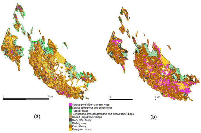
Fig. 4. Map of forest stands in Berezovye Islands resulting (a) from multitemporal data, and (b) from a single hyperspectral image.
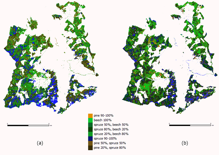
Fig. 5. Map of forest stand in Těšínské Beskydy resulting (a) from multitemporal data, and (b) from a single hyperspectral image.
4 Discussion
The classification using multitemporal MS data had a higher kappa coefficient than did the classification using a single MS or single HS image for Berezovye Island. For Tešínské Beskydy, two of the feature types for multitemporal MS data (K, C) gave lower kappa values than did a single HS image, and classification using a single MS image had the lowest kappa coefficient (Table 5). Even though the single MS image was processed for the most informative phase of vegetation (phenophase 5), during which the maximum reflectance differences between tree species were observed, the classification errors reached 50%. Hill et al. (2010) had reported that the ability to discriminate and map temperate deciduous tree species in airborne multispectral imagery increased using time-series data: from kappa 0.67 for a single image to kappa 0.85 for three images combined (one from autumn, one from the green-up, and one from full-leaf phase). Miyoshi et al. (2017) showed that use of layer stacking from time-series images improved classification, and they achieved an 18% increase in kappa coefficient. Recent studies have used all available cloud-free satellite scenes during a year to classify tree species. For example, Sheeren et al. (2016) analyzed 17 images and Hill et al. (2010) combined three images. Our method revealed selected scenes for classification where the reflectance difference between main tree species was proven as statistically significant. These were the sub-seasons of spring vegetation, first half of summer, and main autumn (leaf fall). Considering the geographical locations and tree species compositions of the study areas, the phenophases distinguished can potentially be utilized for species classification of forests in central Europe and northwestern Russia.
The feature type C that gave the highest kappa for Tešínské Beskydy gave the lowest kappa for multitemporal MS data for Berezovye Islands (Table 5). Every study site will be characterized by more or less uncertainty with regard to determining a specific best method for analyzing reflectance differences. We recommend to use all feature types described (Λ, K, C) and then to choose the one with the highest kappa for a specific forest site.
Most errors were related to the classification of deciduous trees and misclassification of birch as pine (Berezovye Islands), pine as mixture of pine and spruce, and pine as mixture of spruce and beech (Těšínské Beskydy) from the single multispectral image. This is consistent with recent literature. Confusion between deciduous tree species (ash and beech from classification of MS WorldView-2 data) was reported by Waser et al. (2014). Also reported are misclassification of oak as pine from MS Formosat-2 imagery (Sheeren et al. 2016) and misclassification of pine as spruce from MS Sentinel-2 (Immitzer et al. 2016).
The classification results from using a single HS image were close to those when multitemporal MS data were used and the cross-correlation function was applied (Těšínské Beskydy). The main classification error in the case of a single HS image was related to the identification of class “pine” and class “mixture of pine and birch”, with pine being classified incorrectly as mixture of pine and birch (Berezovye Islands). The error can be explained by the fact that the training samples had been obtained from a vegetation map that was more than 10 years old. During this period, a succession of birch forests with pine may have appeared.
The method improved recent forest mapping based on satellite data in regions that were geographically close to the study sites. Pine identification was more accurate using our method (75% in the Berezovye Islands) compared to pine identification from Ikonos satellite data (42% at a location close to Berezovye Islands) (Zhirin et al. 2009). However, spruce identification had lower accuracy in our study in Berezovye Islands (62%) than the 80% achieved by Zhurin et al. (2009). Birch was classified with 66% accuracy in both our study and that of Zhirin et al. (2009). Griffiths et al. (2014) produced a forest types map up to 73% accurate in a Carpathian ecoregion based on Landsat image, whereas our method produced maps up to 81% accurate there.
The proposed method links ground-based observations of phenology to high-resolution land surface phenology products. Using a spectral DB in the proposed method reduces a gap between in situ phenological measurements collected at local scales and land surface phenology metrics (Jimenez et al. 2015). The DB from our study can be a useful addition to publicly open spectral libraries used in vegetation mapping, such as SPECCHIO and EcoSIS.
The proposed methodological approach allows analyzing the phenophases of forest stands and identifying their type using the dynamics of reflectance from satellite data. Use of the method reduces classification error compared to the classification on single satellite images. Species segmentation of forest using the proposed method can potentially be more detailed in comparison with species segmentation from single satellite images. The classification accuracy can be further improved when the method will be applied with a number of new, near-future HS satellite products with high revisit time, like EnMap (Stuffler et al. 2007) and HyspIRI (Devred et al. 2013). The method can potentially be applied for purposes of forest inventory and assessing forest ecosystem stability, where the dynamics of changing species composition comprise one of the main adaptation indicators.
5 Conclusions
The proposed method for tree species classification uses multitemporal multispectral (Landsat OLI) and hyperspectral (Resurs-P) data acquired from determined vegetation periods for two study sites located in the Czech Republic and northwest Russia. The method is based on an original database of spectral features taking into account seasonal variations of tree species spectra. The differences between spectral reflectance of tree species were shown to be statistically significant in the sub-seasons of spring, first half of summer, and main autumn at both study sites. Most of the errors were related to the classification of deciduous tree species and misclassification of birch as pine (northwest Russia site). Pine was classified as mixture of pine and spruce and as a mixture of spruce and beech (Czech site). Tree species are mapped with accuracy up to 80% (northwest Russia site) and 81% (Czech site). The classification using multitemporal multispectral data had a kappa coefficient 1.7 times higher than that from classification using a single multispectral image and a kappa coefficient 1.3 times higher than that from classification using a single hyperspectral image. Potentially, the classification accuracy can be improved by applying multitemporal satellite hyperspectral data for the method, such as the near-future products EnMap and/or HyspIRI with high revisit time.
Acknowledgements
This work was supported by the Ministry of Education, Youth and Sports of the Czech Republic within the CzeCOS program, grant number LM2015061 and by the Ministry of Agriculture of the Czech Republic grant number QK1910150.
References
Arekhi M., Yilmaz O., Yilmaz H., Akyuz Y. (2017). Can tree species diversity be assessed with Landsat data in a temperate forest? Environmental Monitoring and Assessment 11: 189:586. https://doi.org/10.1007/s10661-017-6295-6.
Banskota A., Kayastha N., Falkowski M.J., Wudler M.A., Froese R.E., White J.C. (2014). Forest monitoring using Landsat time series data: A review. Canadian Journal of Remote Sensing 40(5): 362–384. https://doi.org/10.1080/07038992.2014.987376.
Bohn U., Neuhäusl R. (2003). Map of the natural vegetation of Europe. Scale 1: 2.500.000. Landwirtschaftsverlag, Münster.
Boyd D.S., Danson F.M. (2005). Satellite remote sensing of forest resources: three decades of research development. Progress in Physical Cartography 29 (1): 1–26. https://doi.org/10.1191/0309133305pp432ra.
Breiman L. (2001). Random forests. Machine Learning 45(1): 5–32. https://doi.org/10.1023/A:1010933404324.
Brovkina O., Hanuš J., Zemek F., Grigorieva O., Pikl M. (2016). Evaluating the potential of satellite hyperspectral Resurs-P data for forest species classification. The International Archives of the Photogrammetry, Remote Sensing and Spatial Information Sciences, Volume XLI-B1, XXIII ISPRS Congress, 12–19 July 2016, Prague, Czech Republic. p. 443–448. https://doi.org/10.5194/isprs-archives-XLI-B1-443-2016.
Brovkina O., Cienciala E., Zemek F., Lukeš P., Fabianek T., Russ R. (2017). Composite indicator for monitoring of Norway spruce stand decline. European Journal of Remote Sensing 50(1): 550–563. https://doi.org/10.1080/22797254.2017.1372697.
Connette G., Oswald P., Songer M., Leimgrube P. (2016). Mapping distinct forest types improves overall Forest identification based on multi-spectral Landsat Imagery for Myanmar’s Tanintharyi region. Remote Sensing 8(11) article 882. 15 p. https://doi.org/10.3390/rs8110882.
Devred E., Turpie K.R., Moses W., Klemas V.V., Moisan T., Babin M., Toro-Farmer G., Forget M.-H., Jo Y.-H. (2013). Future retrievals of water column bio-optical properties using the Hyperspectral Infrared Imager (HyspIRI). Remote Sensing 5(12): 6812–6837. https://doi.org/10.3390/rs5126812.
Galidaki G., Gitas I. (2014). Mediterranean forest species mapping using classification of Hyperion imagery. Geocarto International 30(1): 48–61. https://doi.org/10.1080/10106049.2014.883439.
Griffiths P., Kuemmerle T., Baumann M., Radeloff V.C., Abrudan I.V., Lieskovsky J., Munteanu C., Ostapowicz K., Hostert P. (2014). Forest disturbances, forest recovery, and changes in forest types across the Carpathian ecoregion from 1985 to 2010 based on Landsat image composites. Remote Sensing of Environment 151: 72–88. https://doi.org/10.1016/j.rse.2013.04.022.
Grigorieva O. (2014). Monitoring of forest degradation from hyperspectral airborne and satellite data. Earth Studies from Space 1: 43–48. [In Russian].
Grigorieva O., Chapursky L. (2012). The problems of creation and content of the database from the coefficients of the spectral brightness of the objects of terrestrial ecosystems. Current Problems in Remote Sensing of the Earth from Space 9(3): 18–25.
Grigorieva O., Saidov A. (2018). Ensemble algorithm of fuzzy clusters for classification of plant communities from satellite hyperspectral data // Conference Proceedings “Problems of military-applied geophysics and control of environment. Saint Petersburg. p. 117–123.
Grigorieva O., Markov A., Saidov A., Terentieva V. (2017). Classification of main forest stand classes based on a series of multi-seasonal many- and hyperspectral remote sensing data. Proceedings of IV International Conference “Regional problems of remote sensing”, Krasnoyarsk. p. 209–212.
Grigorieva O., Kudro D., Saidov A. (2018). An ensemble algorithm for processing hyperspectral data on the basis of training a fuzzy set of clusters in the problem of classifying plant communities. Proceedings of V Russian Scientific Conference “Problems of military applied geophysics and environmental monitoring” SPb, Russia. p. 636–641.
Hájková L., Voženílek V., Tolasz R., Kohut M., Možný M., Nekovář J., Novák M., Richterová D., Stříž M., Vávra A., Vondráková A. (2012). Atlas of phenological conditions in the Czech Republic. Palacky University in Olomouc. 320 p. ISBN 978-80-244-3005-8. [In Czech].
Hill R.A., Wilson A.K., George M., Hinsley S.A. (2010). Mapping tree species in temperate deciduous woodland using time-series multi-spectral data. Applied Vegetation Science 13(1): 86 – 99. https://doi.org/10.1111/j.1654-109X.2009.01053.x.
Hovi A., Raitio P., Rautiainen M. (2017). A spectral analysis of 25 boreal tree species. Silva Fennica 51(4) article 7753. 16 p. https://doi.org/10.14214/sf.7753.
Immitzer M., Vuolo F., Atzberger C. (2016). First experience with Sentinel-2 data for crop and tree species classification in Central Europe. Remote Sensing 8(3) article 166. 27 p. https://doi.org/10.3390/rs8030166.
Jimenez M., Diaz-Delgado R. (2015). Towards a standard plant species spectral library protocol for vegetation mapping: a case study in the Shrubland of Donana National park. ISPRS International Journal of Geo-Information 4(4): 2472–2495. https://doi.org/10.3390/ijgi4042472.
Lausch A., Erasmi S., King J.D., Magdon P., Heurich M. (2016). Understanding forest health with remote sensing -part i – a review of spectral traits, processes and remote-sensing characteristics. Remote Sensing 8(12) article 1029. 44 p. https://doi.org/10.3390/rs8121029.
Leningrad Region. Nature and economy (1958). Leningrad: lenizdat. 343 p. [In Russian].
Markov A., Grigorieva O., Saidov A., Mochalov V., Zhukov D. (2015). Software package for thematic processing of satellite hyperspectral and multispectral data. Geomatics 1: 32–37. [In Russian].
McRoberts R.E., Tomppo E.O. (2007). Remote sensing support for national forest inventories. Remote Sensing of Environment 110(4): 412–419. https://doi.org/10.1016/j.rse.2006.09.034.
Michalko J. (1986). Geobotanic map CSSR. Veda, Bratislava. 186 p.
Miyoshi G.T., Imai N.N., de Moraes M.V.A., Tommaselli A.M.G., Nasi R. (2017).Time series of images to improve time-series classification. SPRS archives, Volume XLII-3/W3. http://doi.org/10.5194/isprs-archives-XLII-3-W3-123-2017.
Pax-Lenney M., Woodcock C.E., Macomber S.A., Gopal S., Song C. (2001). Forest mapping with a generalized classifier and Landsat TM data. Remote Sensing of Environment 77(3): 241–250. https://doi.org/10.1016/S0034-4257(01)00208-5.
Saidov A. (2012). The structure of a relation database of main types of landscape reflectance spectra and its software-based GIS. Current Problems in Remote Sensing of the Earth from Space 9(3): 70–74.
Sasaki N., Takejima K., Kusakabe T., Sweda T. (2001). Forest cover classification using Landsat TM data for areal expansion of line LAI estimate generated through airborne laser profile. Polar Bioscience 14: 110–121.
Schowengerdt R. (2006). Remote Sensing: models and methods for image processing. Academic Press. 560 p.
Shafri H.Z.M., Suhaili A., Mansor S. (2007). The performance of Maximum Likelihood, Spectral Angle Mapper, Neural Network and Decision Tree classifiers in hyperspectral image analysis. Journal of Computer Science 3(6): 419–423. https://doi.org/10.3844/jcssp.2007.419.423.
Shataee S., Kellenberger T., Darvishsefat A.A. (2004). Forest types classification using ETM+ data in the north of Iran/ comparison of object-oriented with pixel-based classification techniques, XX ISPRS Congress Commission PS, Working Group VII/1.
Sheeren D., Fauvel M., Josipovic V., Lopes M., Planque C., Willm J., Dejoux J.-F. (2016). Tree species classification in temperate forests using Formosat-2 satellite image time series. Remote Sensing 8(9) article 734. 29 p. https://doi.org/10.3390/rs8090734.
Stanek J., Zatloukal V., Kubu M., Matejcek J., Skoblik J., Vasicek J., Kopecny K. (1997). Forest law in theory and practice. The full regulations with comments. p. 229–392. [In Czech].
Stepanchikova I.S., Schiefelbein U., Alexeeva N.M., Ahti T., Kukwa M., Himelbrant D.E., Pykälä J. (2011). Additions to the lichen biota of Berezovye Islands, Leningrad Region, Russia. Folia Cryptogamica Estonica 48: 95–106.
Stuffler T., Kaufmann H., Hofer S., Forster K.P., Schreier G., Müller A., Eckardt A., Bach H., Penne B., Benz U., Haydn R. (2007). The EnMAP hyperspectral imager – an advanced optical payload for future applications in Earth observation programmes. Acta Astronautica 61(1–6): 115–120. https://doi.org/10.1016/j.actaastro.2007.01.033.
Terebizh V.J. (2005). An introduction to the statistical theory of inverse problems. M.: PHISMALIT. 376 p. [In Russian].
Tigges J., Lakes T., Hostert P. (2013). Urban vegetation classification: benefits of multitemporal RapidEye satellite data. Remote Sensing of Environment 136: 66–75. https://doi.org/10.1016/j.rse.2013.05.001.
Transon J., d’Andrimont R., Maugnard A., Defourny P. (2017). Survey of hyperspectral earth observation applications from space in the Sentinel-2 context. Remote Sensing 10(157): 1–32. https://doi.org/10.3390/rs10020157.
Volkova Е.А., Glazkova Е.А., Isachenko G.А., Chramtsov V.N. (2016). Natural environment and ecological diversity of the archipelago Berezovye Islands (Gulf of Finland). Saint Petersburg. 328 p. [In Russian].
Waser L.T., Küchler M., Jütte K., Stampfer T. (2014). Evaluating the potential of WorldView-2 data to classify tree species and different levels of Ash mortality. Remote Sensing 6: 4515–4545. https://doi.org/10.3390/rs6054515.
Zhirin V., Knyazeva S. (2009). Estimation of the possibilities of forest forming species recognition on the base of IKONOS space image. Current Problems in Remote Sensing of the Earth from Space 2(6): 373–379.
Zhou T., Li Z., Pan J. (2018). Multi-feature classification of multi-sensor satellite imagery based on dual-polarimetric Sentinel-1A, Landsat-8 OLI, and Hyperion images for urban land-cover classification. Sensors 18(373): 1–20. https://doi.org/10.3390/s18020373.
Total of 44 references.
