Ana de Lera Garrido  ,
Terje Gobakken,
Hans Ole Ørka,
Erik Næsset,
Ole M. Bollandsås
,
Terje Gobakken,
Hans Ole Ørka,
Erik Næsset,
Ole M. Bollandsås
Estimating forest attributes in airborne laser scanning based inventory using calibrated predictions from external models
de Lera Garrido A., Gobakken T., Ørka H. O., Næsset E., Bollandsås O. M. (2022). Estimating forest attributes in airborne laser scanning based inventory using calibrated predictions from external models. Silva Fennica vol. 56 no. 2 article id 10695. https://doi.org/10.14214/sf.10695
Highlights
- Three approaches to calibrate temporal and spatial external models using field observations from different numbers of local plots are presented
- Calibration produced satisfactory results, reducing the mean difference between estimated and observed values in 89% of all trials
- Using few calibration plots, ratio-calibration provided the lowest mean difference
- Calibration using 20 plots gave comparable results to a local forest inventory.
Abstract
Forest management inventories assisted by airborne laser scanner data rely on predictive models traditionally constructed and applied based on data from the same area of interest. However, forest attributes can also be predicted using models constructed with data external to where the model is applied, both temporal and geographically. When external models are used, many factors influence the predictions’ accuracy and may cause systematic errors. In this study, volume, stem number, and dominant height were estimated using external model predictions calibrated using a reduced number of up-to-date local field plots or using predictions from reparametrized models. We assessed and compared the performance of three different calibration approaches for both temporally and spatially external models. Each of the three approaches was applied with different numbers of calibration plots in a simulation, and the accuracy was assessed using independent validation data. The primary findings were that local calibration reduced the relative mean difference in 89% of the cases, and the relative root mean squared error in 56% of the cases. Differences between application of temporally or spatially external models were minor, and when the number of local plots was small, calibration approaches based on the observed prediction errors on the up-to-date local field plots were better than using the reparametrized models. The results showed that the estimates resulting from calibrating external models with 20 plots were at the same level of accuracy as those resulting from a new inventory.
Keywords
forest inventory;
LIDAR;
calibration;
area-based approach;
spatial transferability;
temporal transferability
-
de Lera Garrido,
Faculty of Environmental Sciences and Natural Resource Management, Norwegian University of Life Sciences, P.O. Box 5003, NO-1432 Ås, Norway
E-mail
ana.de.lera@nmbu.no
- Gobakken, Faculty of Environmental Sciences and Natural Resource Management, Norwegian University of Life Sciences, P.O. Box 5003, NO-1432 Ås, Norway E-mail terje.gobakken@nmbu.no
- Ørka, Faculty of Environmental Sciences and Natural Resource Management, Norwegian University of Life Sciences, P.O. Box 5003, NO-1432 Ås, Norway E-mail hans-ole.orka@nmbu.no
- Næsset, Faculty of Environmental Sciences and Natural Resource Management, Norwegian University of Life Sciences, P.O. Box 5003, NO-1432 Ås, Norway E-mail erik.naesset@nmbu.no
- Bollandsås, Faculty of Environmental Sciences and Natural Resource Management, Norwegian University of Life Sciences, P.O. Box 5003, NO-1432 Ås, Norway E-mail ole.martin.bollandsas@nmbu.no
Received 7 January 2022 Accepted 4 April 2022 Published 25 April 2022
Views 56628
Available at https://doi.org/10.14214/sf.10695 | Download PDF

Supplementary Files
1 Introduction
Modern forest management inventories (FMI) rely on predictive models of stand attributes that are dependent on metrics calculated from airborne laser scanning (ALS). Field measurements and ALS data are typically acquired the same year within the geographical boundaries of each specific FMI, and the prediction models are constructed and applied specifically for each FMI. This ensures that metrics from the same ALS instrument are used for both model construction and in the prediction phase. Ideally, the models should be constructed with field data that cover the range of the stand attributes in the population to avoid extrapolation in the prediction phase, which may lead to systematic prediction errors for the extreme values of the population. Furthermore, models constructed with field- and ALS data from a different population are prone to produce predictions with systematic errors across the whole range of the target population.
Several studies have shown that the properties of ALS point clouds vary between acquisitions due to several factors related to the sensor such as output energy of the laser, detection method of the reflected energy, or pulse width (Næsset 2009). The instrument algorithms used to detect and trigger a return will also influence the properties of the point cloud (Wagner et al. 2004). Furthermore, it has been shown that acquisition parameters such as flying altitude, scan angle, or pulse repetition frequency (PRF) also affect the point cloud properties (Hopkinson 2007; Morsdorf et al. 2007). For example, changes in PRFs can affect the pulse penetration into the canopy and may therefore cause shifts in the canopy height distributions, and higher flight altitude may decrease the proportion of pulses with multiple returns (Næsset 2004)
Another factor that can introduce noise in ALS-based inventories is variations of forest structure, e.g., the shape of stems and tree crowns (Ørka et al. 2010). Growth conditions that affect forest structure and allometry vary between different geographical regions because of variations in local climate and soil properties. In the context of area-based FMIs as described here, it means that the structural signatures of the ALS point clouds from forests of identical volumes, biomass, mean heights, etc., can be different. Thus, predictions by means of a model constructed on data from outside the target population (external model) might yield systematic prediction errors.
Despite apparent challenges, external models can be beneficial, for example, when sufficient field data for model construction is lacking for an area where an inventory is carried out. It is also an alternative to either reduce or omit the collection of field data in the area of interest to reduce the total cost of the inventory if relevant external models are available. However, such strategies require documentation of suitability of the external model for the target population or field observations within the target population to be used for verification or calibration purposes.
Several studies have assessed the effect of including field observations from the target population to obtain more accurate predictions from models mainly constructed on external data. Latifi and Koch (2012) explored the potential of using data from an auxiliary inventory to provide estimates of volume, above-ground biomass, and stem number. They combined the auxiliary inventory plots (120) with varying numbers of sample plots drawn from the target population (0 to 200 plots) using random forest and most similar neighbors. They concluded that the inclusion of plots from the target population improved the predictions and reduced the systematic errors. Kotivuori et al. (2016) tested the effect on prediction accuracy of nationwide models if they were calibrated with regional plots using mixed-effects modeling. Overall, local calibration improved the predictions for all inventory areas included in their study. Kotivuori et al. (2018) fitted new nationwide models for stem volume and examined different calibration scenarios to minimize the errors caused by geographical variation in forest structure. They applied calibration of the national model with 1) additional predictor variables describing local climate and forest conditions, 2) the 200 geographically nearest sample plots from other inventory projects, and 3) ratios between volume estimates from the multi-source national forest inventory of Finland and uncalibrated estimates for the target inventory area. The best calibration scenario was obtained by adding degree days, the standard deviation of precipitation, and the proportion of birch as additional variables in the nationwide model. All these studies focused on spatially external models and showed that calibration using local information improved their performance. Most of the studies combined many plots from the target area with external plots in the model construction. However, the accuracy of calibrated predictions did not outperform those that resulted from using models calibrated entirely on local data.
The benefit of external models is undeniable if they achieve higher accuracy than an ordinary local ALS inventory. However, even though external models might not perform as well as models constructed on local data, their application might still be beneficial. Since field data collection is a costly part of an FMI, reducing or even omitting it for the target population will reduce the total costs (Breidenbach et al. 2008; Suvanto and Maltamo 2010). External models are a viable option if this cost reduction exceeds the cost of potentially having inferior inventory information that leads to poorer management decisions (Mäkinen et al. 2012; Ruotsalainen et al. 2019). The local plots can be used together with external plots to construct a model used for prediction, or the local plots can be used to estimate and correct the systematic error that might arise from an entirely external model.
This study aimed to use a limited number of local plot observations to estimate systematic errors and calibrate external model predictions. We analyze three different calibration strategies applied to spatially and temporally external models. Our forest attributes of interest were volume, stem number, and dominant height. The external models were applied in three target areas and calibrations were carried out using different numbers of local plots. The predictions were aggregated to estimates for small stands, and accuracy and precision were evaluated by assessing the differences between estimates and field reference values. We assessed the effect of calibration by comparing the results against the uncalibrated predictions. Finally, we compared the results against those of ordinary ALS inventories from the respective target areas and assessed the success by the frequency of the calibration approaches improving the results.
2 Materials
2.1 Study areas
The study was conducted within three districts in boreal forest in southeastern Norway: Nordre Land, Krødsherad, and Hole, hereafter referred to as districts A, B, and C, respectively (Fig. 1). The distance between the districts range between 39 and 102 km, and all three belong to the same climate zone. The main tree species in districts A and B are Norway spruce (Picea abies [L.] Karst.) and Scots pine (Pinus sylvestris L.), and district C is a Norway spruce-dominated area. The altitudes above sea level range from 130 to 900 m.
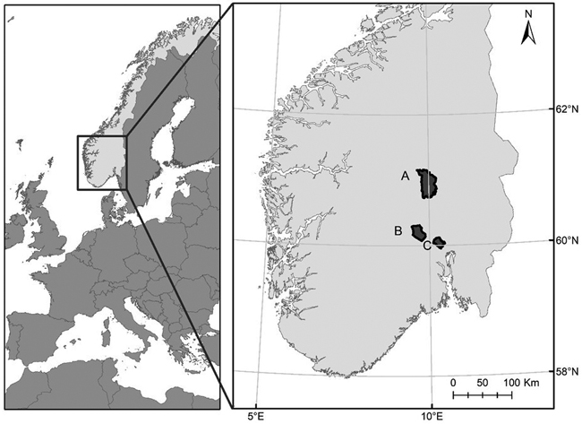
Fig. 1. Location of the three districts used in the study: Nordre Land (A), Krødsherad (B), and Hole (C).
2.2 Field measurements
Field data were collected as part of operational forest management inventories carried out during the years 2002, 2003, and 2005 (labeled T1) for districts A, B, and C, respectively, and as part of remeasurements of the same areas during 2016 (district B) and 2017 (districts A, B, and C) (labeled T2).
The dominant tree species, site productivity classes (SI), age, and development class were interpreted from aerial images for each district. Based on the photo interpretation, stands were delineated and stratified, and circular training plots were spatially distributed according to stratified systematic sampling designs at T1. The same training plots were re-measured at T2. Due to differences in the stratification criteria between the districts, we limited the scope of this study to mature stands dominated by pine or spruce, which were common for all districts.
Apart from the training plots used for modelling, the study also comprised validation plots for each district. For districts A and C, validation plots were circular with size 1000 m2 and each of them was concentric to one of the training plots. For district B, the plots were quadratic with size ~3720 m2 (61 × 61 m) with locations independent of the training plots. Table 1 shows an overview of the number and size of plots for the different districts.
| Table 1. Overview of the districts (A, B, and C) and their measured plots used in the study at two points in time (T1 and T2). | |||||||||||||||
| Training plot T1 | Training plot T2 | Validation plot T2 | |||||||||||||
| District | Elev. | Year | n | ps | P | Year | n | ps | P | n | ps | P | |||
| A | 140–900 | 2003 | 193 | 250 | 0.73 | 2017 | 170 | 250 | 0.64 | 25 | 1000 | 0.28 | |||
| B | 130–660 | 2001 | 74 | 232.9 | 0.39 | 2016/17 | 75 | 232.9 | 0.35 | 43 | 3721 | 0.44 | |||
| C | 240–480 | 2005 | 78 | 250 | 1 | 2017 | 43 | 250 | 1 | 22 | 1000 | 1 | |||
| Elev. = elevation above sea level (m); n = number of plots; ps = plot size (m2); P = proportion of spruce-dominated plots. | |||||||||||||||
On each training plot, trees with diameter at breast height (dbh) ≥ 10 cm, were calipered. Sample trees were selected for the pure purpose of measuring tree heights and the heights were measured using a Vertex hypsometer. Sample trees were selected with a probability proportional to stem basal area using a relascope. The sampling intensity was proportional to the reciprocal of stand basal area so that approximately 10 trees per plot would be selected for height measurements. On plots with fewer than 10 trees, all trees were selected as sample trees. For circular validation plots, tree measurements were similar to those of the training plots. In district B, where the validation plots were square, the dbh measurements were as described above, but the selection of sample trees was carried out according to the accumulation of basal area in 2-cm diameter classes during dbh measurements.
Field measurements were used to calculate plot-level dominant height (Ho), stem number per hectare (N), and volume per hectare (V). We predicted the volume and height for all calipered trees employing ratio estimation (Cochran 1977, p. 151) as described in Ørka et al. (2018). Ho was calculated as the mean predicted height of the n largest trees according to dbh, where n was calculated as 100 × (plot size/hectare). At T2, field and ALS data were acquired at different years. Field data were back-casted using a correction factor (de Lera Garrido et al. 2020) to match the value at the time point of the ALS acquisition. A summary of the ground reference data is shown in Fig. 2.
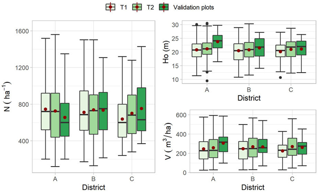
Fig. 2. Box plots showing the distribution of the field plot attributes per district (dominant heigh (Ho), volume (V), and stem number (N)) for the training plots measured at two points in time (T1 and T2) and the validation plots measured at T2. The mean value is indicated with a red dot.
2.3 Airborne laser scanning data
ALS data were acquired under leaf-on conditions at two points in time for all districts. Table 2 shows the applied instruments and acquisition parameters. Following standard routines, the initial ALS processing was carried out by the contractors. The ALS returns were first classified into ground and non-ground returns, and then terrain surface models were created from the ground returns using a triangular irregular network (TIN). The height above the TIN was then calculated for each of the non-ground returns.
| Table 2. Summary of ALS instrument specifications and flight acquisition parameter settings for the different districts (A, B and C). | ||||||
| District | year | Instrument | Mean flying altitude (m) | Pulse repetition frequency (kHz) | Scanning frequency (Hz) | Mean point density (pts m–2) |
| First acquisition (T1) | ||||||
| A | 2003 | Optech ALTM 1233 | 800 | 33 | 40 | 1 |
| B | 2001 | Optech ALTM 1210 | 650 | 10 | 30 | 1 |
| C | 2005 | Optech ALTM 3100 | 2000 | 50 | 38 | 1 |
| Second acquisition (T2) | ||||||
| A | 2016 | Riegl LMS Q-1560 | 2900 | 400 | 100 | 4 |
| B | 2016 | Riegl LMS Q-1560 | 1300 | 534 | 115 | 12 |
| C | 2016 | Riegl LMS Q-1560 | 1300 | 534 | 115 | 10 |
For consistency between the acquisitions and because the heights above the TIN of the last returns are more affected by the ALS instrument properties than the heights of the first returns (Næsset 2005), we computed ALS metrics from the first return category only. This category includes “first of many” and “single” returns. We calculated canopy height ALS metrics for each plot using returns with a height value > 2 m. The metrics were percentiles of the height distributions (H10, H20, …, H90), the arithmetic mean height (Hmean), maximum height (Hmax), standard deviation (Hsd), and coefficient of variation (Hcv) of return heights. For the canopy density metrics, we divided the vertical range between 2 m and the 95th percentile into 10 bins of equal length. Then we calculated the density metrics (D0, D1, ..., D9) as the proportion of returns above the lower limit of each bin and the total number of returns.
For prediction purposes and to match the size of the training plots, we divided the validation plots into smaller segments. In districts A and C, this division was into quadrants of 250 m2 each. In district B, the segments were 16 squares of approximately 15.26 m × 15.26 m. ALS metrics were calculated for prediction purposes for each individual segment.
3 Methods
Fig. 3 summarizes graphically the main analysis performed in the methodology and explained in the following sections.
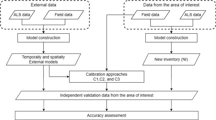
Fig. 3. Flowchart showing the main analysis of the methodology to calibrate forest attribute predictions from external models.
3.1 Differences in the forest attribute cumulative distribution between districts
Before using an external model, an assessment of the similarity between reference and target sites should be made, although this is not always possible using observed field data. However, prior knowledge of tree species distribution and factors that affect tree allometry should be considered. Although the three districts in this study are in geographically proximity and belong to the same climatic region, we tested the similarity of the different field data sets with a two-sample Kolmogorov-Smirnov test (KS) that analyzed if two underlying distributions are the same. We compared the empirical cumulative distribution functions of each forest attribute in all datasets, and we calculated the maximum vertical distance (D) between the cumulative distributions of the datasets. KS test returns the p-value of the test to determine if the two distributions differ significantly.
3.2 External models
To predict Ho, N, and V, we constructed two types of external models: 1) models labeled “temporal models” constructed on data from each district at T1 to be applied at T2 in the same district; and 2) models labeled “spatial models” constructed on data from district A at T2 to be applied in districts B and C at T2. We decided to construct the spatial external model from district A because this district was the one capturing the widest range of variation of the forest attributes included in this study. Although models combining temporally and spatially external data could have also been carried out, we decided to compare the use of the two types of data sources exclusively.
The models were constructed using an automatic procedure. To select the explanatory variables, we first created linear models for each forest attribute, for which both response and explanatory variables (ALS metrics) were log-transformed. We performed a variable search with the stepwise algorithm ‘regsubsets’ from the leaps package in R (Lumley and Miller 2020), and we limited the maximum number of explanatory variables to three. In addition to the maximum of three ALS metrics, a dummy variable (ts), representing dominant tree species (pine: ts = 0, spruce: ts = 1), was added to the models constructed for districts A and B.
The resulting alternative linear models for each response, district, and inventory occasion were ranked according to the Bayesian information criterion (BIC) after models with variance inflation factor greater than 5 had been discarded. The explanatory variables of the linear log-log models with the lowest BIC were used on the original scale as explanatory variables for constructing nonlinear models. The nonlinear models (Eq. 1) were then fitted using the ‘nls’ function with the Gauss-Newton algorithm from the stats package, using the model coefficient estimates of the corresponding linear log-log models as starting values. Finally, residuals plots were used to visually check that heteroscedasticity was not a major problem.
![]()
where ![]() is the response variable, a, b, and c are the selected explanatory variables, β0, β1, β2, β3 and β4 are the parameters to be estimated, ts is the dummy variable and ε the error term.
is the response variable, a, b, and c are the selected explanatory variables, β0, β1, β2, β3 and β4 are the parameters to be estimated, ts is the dummy variable and ε the error term.
3.3 Calibration approaches
We applied three common calibration approaches that only required the external model, not the external field information, to eliminate or reduce the potential systematic deviations of using external models. For all approaches (explained below), different numbers of field training plots (in this context labeled “calibration plots”) were used to perform the calibration. Calibration plots were selected using simple random sampling with replacement. For each approach and number of plots used, the procedure was repeated 1000 times with an independent sample drawn each time. For consistency between all districts, the number of calibration plots ranged between 10 and 60, even in district C which only had 43 plots measured at T2. However, we accounted for this limitation by using sampling with replacement. In districts A and B, the proportions of pine- and spruce dominated plots for the selection were forced to be equal, i.e., 50% for each.
In the approaches labeled C1 and C2, predictions were calibrated using the observed prediction errors of the external models on the calibration plots. For C1 ratios (r) between field references and predictions of the calibration plots were calculated and used as multiplicators to the external predictions on the validation plots. For C2 linear prediction models for the field reference values were constructed with the external prediction as explanatory variable.
In C1, we estimated r according to the principle of «ratio-of-means» (Cochran, 1977, p. 151) as the ratio between the sum of observed and predicted values. The corrected predictions ![]() were then calculated as:
were then calculated as:
![]()
where ![]() is the uncalibrated prediction using the external model.
is the uncalibrated prediction using the external model.
In C2, the prediction model for the field-observed response ![]() with the external prediction
with the external prediction ![]() as the explanatory variable was specified as:
as the explanatory variable was specified as:
![]()
where α0 and α1 are parameters to be determined by regression analysis and ε is the error term. Corrected predictions ![]() for the validation plots were calculated as:
for the validation plots were calculated as:
![]()
In the third approach (labeled C3), the calibration plots were used to construct models using the explanatory variables already selected for the external model. In this reparameterization, we preserved the mathematical form of the external model and the explanatory variables but updated the model parameters. The rationale for applying this approach was that the explanatory variables used in the external model were selected on data sets large enough that sufficiently enables a proper variable selection. Thus, we assumed that although the temporal and spatial differences affect the model’s validity, the explanatory variables would still be appropriate. Therefore, using a reduced number of calibration plots to update the model coefficients could be sufficient to correct the estimates.
3.4 New inventory
To compare with the calibrated predictions, we constructed new local prediction models (labeled NI) using different numbers of training plots from T2 (from 10 to 60). We used simple random selection with replacement for the model construction, and we repeated the procedure 1000 times for each district, performing a new automatic variable selection in each iteration. The rationale for using selection with replacement was, as for the calibration approaches, to allow for greater variation between samples of each iteration in the simulation. An ordinary FMI typically uses between 40 and 50 field plots per stratum (Næsset 2014). In our most comprehensive alternative, we used 60 plots (30 per stratum) because we wanted to keep the same number of plots used in the calibration approaches. Even if the number is smaller than in an ordinary inventory, we consider that the inventory constructed with 60 plots (denoted NI60) resembles a new ordinary inventory and can be used as a benchmark.
3.5 Accuracy assessment
The models were applied to the validation plots to obtain estimates of Ho, V, and N. Then, we calculated and assessed the accuracy and precision of the external models for both the uncalibrated predictions and after applying the calibration procedures.
The predictions for the segments of the validation plots were aggregated to estimates as means of the quadrants of the circular plots (districts A and C) or means of the 16 squares (district B). To assess the accuracy and precision, the relative mean difference (MD%) and the relative root mean squared error (RMSE%) were calculated,
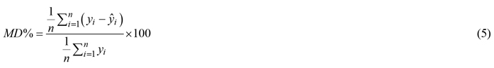
where n is the number of validation plots, ![]() is the field reference value of either Ho, V or N for plot i, assumed to be acquired without error, and
is the field reference value of either Ho, V or N for plot i, assumed to be acquired without error, and ![]() is the estimated value for plot i.
is the estimated value for plot i.
For the uncalibrated predictions of the external models, we applied an ordinary bootstrap resampling with 1000 replicates. For each resample of validation plots, new MD% and RMSE% values are calculated, and with the distribution of the obtained statistics, we construct the nonparametric 95% confidence interval (CI).
Although MD% and RMSE% are widely applied uncertainty metrics, for a more detailed description of the uncertainty, we constructed as a complementary measure a linear parametric error model (Eq. 7), with the estimated ![]() and observed
and observed ![]() values as dependent and explanatory variables, respectively. The parameter estimates of such models describe and quantify the error structures concisely and illustrate how the error components vary across the field reference values (Persson and Ståhl 2020). The model was fitted with ordinary least squares regression and consisted of three parameters (λ0, λ1, and εm) that describes the error structure of the plot level estimates. λ0 represents the systematic error, λ1 represents how the error varies across the range of field reference values (it can be considered a scaling factor), and the size of the random error terms, εm can be quantified by their standard deviation (σεm).
values as dependent and explanatory variables, respectively. The parameter estimates of such models describe and quantify the error structures concisely and illustrate how the error components vary across the field reference values (Persson and Ståhl 2020). The model was fitted with ordinary least squares regression and consisted of three parameters (λ0, λ1, and εm) that describes the error structure of the plot level estimates. λ0 represents the systematic error, λ1 represents how the error varies across the range of field reference values (it can be considered a scaling factor), and the size of the random error terms, εm can be quantified by their standard deviation (σεm).
![]()
The median values of the 1000 individual values of MD%, RMSE% from the simulations, were used to assess the accuracy of the calibration approaches and NI. The median of the parameters of the error structure model were also calculated. They were labeled ![]() respectively. Since the validation plots were not independent from the calibration plots in districts A and C, we performed leave-one-out cross-validations (loocv) for these areas.
respectively. Since the validation plots were not independent from the calibration plots in districts A and C, we performed leave-one-out cross-validations (loocv) for these areas.
Finally, to compare the results from the calibration approaches against a new ordinary inventory, we calculated the percentages of cases where the calibration improved the results of NI60. We grouped the results in different ways (e.g., considering each approach individually or all approaches as a whole). The percentages were relative to the total number of approaches considered, which differs between the different ways of grouping the results. The percentage of cases where the results were improved were labeled “success rate.”
4 Results
4.1 Differences in the forest attribute cumulative distribution between districts
Table 3 shows the distances (D) between the empirical distributions of the field data and the corresponding p-values estimated by the two-sample KS test. p-values < 0.05 indicate that D is large enough to consider the two distributions to be different. The largest D values were found for district A with a p-value < 0.05 for the forest attributes Ho (T1 and T2) and V (T1), showing that the populations differ in median, variability, or the shape of the distribution. For the rest, the KS test showed no significant differences between the distribution for the two pairs of samples.
| Table 3. Results of the two-sample Kolmogorov-Smirnov test between the training field plots measured at two points in time (T1 and T2) and the validation plots measured at T2 in the three districts (A, B and C). | ||||||||||
| Validation district A (T2) | Validation district B (T2) | Validation district C (T2) | ||||||||
| District | Statistic | H | V | N | H | V | N | H | V | N |
| A (T1) | D | 0.39 | 0.28 | 0.22 | ||||||
| p-value | 0.002 | 0.04 | 0.22 | |||||||
| A (T2) | D | 0.36 | 0.24 | 0.26 | 0.14 | 0.17 | 0.12 | 0.13 | 0.20 | 0.18 |
| p-value | 0.005 | 0.14 | 0.10 | 0.43 | 0.22 | 0.69 | 0.86 | 0.41 | 0.55 | |
| B (T1) | D | 0.19 | 0.21 | 0.21 | ||||||
| p-value | 0.25 | 0.14 | 0.20 | |||||||
| B (T2) | D | 0.17 | 0.15 | 0.10 | ||||||
| p-value | 0.37 | 0.51 | 0.93 | |||||||
| C (T1) | D | 0.22 | 0.28 | 0.19 | ||||||
| p-value | 0.38 | 0.14 | 0.52 | |||||||
| C (T2) | D | 0.08 | 0.24 | 0.15 | ||||||
| p-value | 1 | 0.37 | 0.88 | |||||||
4.2 Accuracy of the uncalibrated external models
Between one and three response variables were selected for the external models, always one height metric and in addition one or two density metrics. The accuracies obtained in the model validation of the external models (uncalibrated predictions) are shown in Table 4. Independent of the district and type of external model, the smallest values of MD% and RMSE%, were obtained for the Ho models, and the largest for the models for N. The 95% bootstrapped confidence intervals were relatively wide for both MD% and RMSE%, especially for N and V. In eight of 15 cases the confidence intervals of the MD% included zero. Values of λ1 ranged from 0.52 to 1.11, where V was the attribute with λ1 values closest to 1. Overall, without calibration, the predictions using the temporally external models were more accurate than those obtained using the spatially external models. Only in district C the MD% of the predictions of the spatially external model (H and V) indicated better accuracy compared to the temporally external predictions.
| Table 4. Selected predictors and validation results for temporally and spatially externally models for Ho, V and N. RMSE% and relative mean difference of predictions (MD%) with corresponding 95% confidence intervals (CIRMSE, CIMD), and error model parameters (λ0, λ1, and σεm) were calculated after application of the models on validation datasets from districts A, B, and C. | |||||||||
| Predictors* | RMSE% | CIRMSE | MD% | CIMD | λ0 | λ1 | σεm | ||
| Temporal | |||||||||
| A | Ho | H90, D0 | 8.3 | 5.8, 10.9 | –2.0 | –5.1, 1 | 7.0 | 0.7 | 1.5 |
| V | H70, D0 | 22.6 | 16.1, 29.1 | 9.1 | –0.1, 17.4 | 90.8 | 0.8 | 62.0 | |
| N | Hmax, D0, D9 | 25.8 | 19.0, 33.1 | 2.1 | –8.4, 12.4 | 267.5 | 0.6 | 135.0 | |
| B | Ho | H90, D5 | 5.1 | 3.7,6.5 | 0.4 | –1.2, 1.9 | 4.1 | 0.8 | 0.9 |
| V | H80, D0 | 15.6 | 9.8, 22.0 | 5.1 | 0.6, 9.6 | 49.7 | 0.9 | 37.0 | |
| N | H80, D1 | 26.8 | 19.2, 34.8 | –7.1 | –13.9, –0.1 | 320.8 | 0.5 | 125.8 | |
| C | Ho | H90, D0, D7 | 4.5 | 3.3, 5.8 | 2.0 | 0.3, 3.8 | 2.3 | 0.9 | 0.8 |
| V | H40, D4 | 19.0 | 11.7, 26.9 | 5.9 | –2.2, 14 | 52.5 | 0.9 | 44.4 | |
| N | H90, D4 | 25.1 | 17.5, 34 | –9.9 | –18.1, –1.7 | 285.3 | 0.5 | 100.3 | |
| Spatial | |||||||||
| B | Ho | H90 | 5.3 | 3.8, 6.7 | 1.5 | –0.1, 3.1 | 5.2 | 0.8 | 0.7 |
| V | H90, D0, D8 | 21.2 | 14.1, 28.9 | 11.4 | 6.5, 16.6 | 1.7 | 1.1 | 46.6 | |
| N | Hmax, H30, D0 | 26.0 | 17.4, 34.4 | 12.5 | 4.3, 20.1 | 266.8 | 0.8 | 158.8 | |
| C | Ho | H90 | 5.0 | 3.5, 6.6 | –0.5 | –2.3, 2.0 | 4.1 | 0.8 | 0.8 |
| V | H90, D0, D8 | 19.8 | 10.5, 29.1 | 4.7 | –3.3, 12.4 | 48.9 | 0.9 | 46.0 | |
| N | Hmax, H30, D0 | 26.3 | 18.5, 34.6 | 15.5 | 5.5, 25.4 | 291.7 | 0.8 | 145.9 | |
| * H30, H40, H70, H80 and H90 = 30, 40, 70, 80 and 90 percentiles of the laser canopy heights; Hmax = maximum laser canopy height; D0, D1, … D9 = canopy densities corresponding to the proportions of laser returns above each bin # 0, 1, … 9, respectively, to total number of returns (see text). | |||||||||
4.3 Accuracy of the calibrations approaches and new inventory with different number of calibration plots
For each district and forest attribute, the MD% and RMSE% based on the calibration approaches and NI are presented as separate graphical figures. Figs. 4–6 show examples for each district and forest attribute, and the rest of the figures can be found in Supplementary file S1. Each figure displays the distributions of MD% and RMSE% from the 1000 iterations as boxplots for each number of calibration plots used. Results from the different approaches are displayed in different colors, and the mean relative difference obtained from uncalibrated predictions using external models as horizontal dashed lines with the corresponding bootstrapped 95% CI as a colored area around the respective lines. Due to outliers and to have a better visualization of the boxplots, the figures are not displayed in their full extent. This visualization choice did not affect the underlying data.
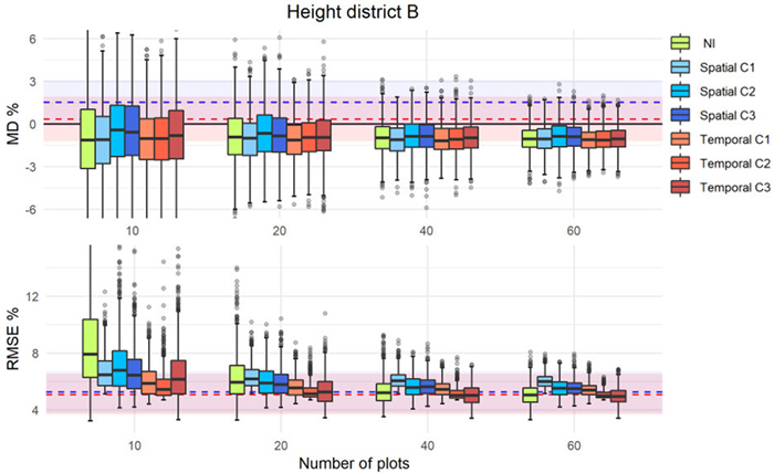
Fig. 4. MD% and RMSE% distributions from 1000 iterations in simulations of different calibration approaches (as boxplots) using external prediction models of dominant height in district B. The MD% (upper panel) and RMSE% (lower panel) of uncalibrated external predictions are displayed with dashed lines (blue = spatial, red = temporal) with corresponding confidence intervals displayed as colored areas around the respective lines.
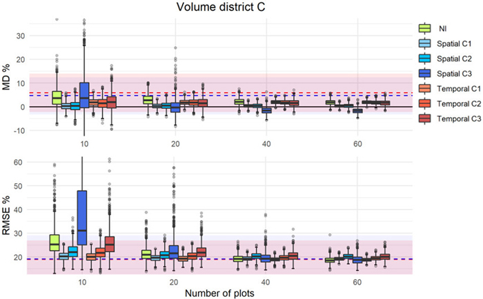
Fig. 5. MD% (upper) and RMSE% (lower) distributions from 1000 iterations in simulations of different calibration approaches (as boxplots) using external prediction models of volume in district C. The uncalibrated external predictions are displayed with dashed lines (blue = spatial, red = temporal) with the corresponding confidence intervals as colored areas around the respective lines.
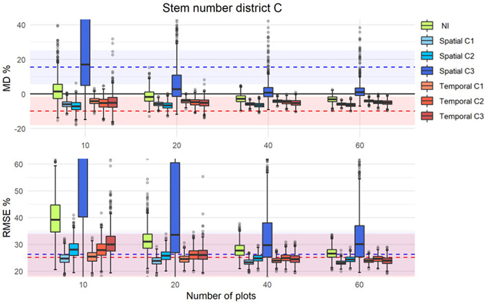
Fig. 6. MD% and RMSE% distributions from 1000 iterations in simulations of different calibration approaches (as boxplots) using external prediction models of stem number in district C. The MD% (upper panel) and RMSE% (lower panel) of uncalibrated external predictions are displayed with dashed lines (blue = spatial, red = temporal) with corresponding confidence intervals displayed as colored areas around the respective lines.
The results showed that the calibration, even with a small number of calibration plots, improved the accuracy of the predictions of the external models. With only 10 calibration plots, ![]() improved and was closer to zero. However, in some cases and independently of the number of plots used, the uncalibrated external model was the best (see Fig. 4). Overall, the interquartile range of the boxplots were inside the CIs of the uncalibrated predictions of the external models, and with increasing number of calibration plots, the precision was improved as indicated by more narrow ranges of the boxplots and a decreasing number of outliers. For the calibration approach C1, the
improved and was closer to zero. However, in some cases and independently of the number of plots used, the uncalibrated external model was the best (see Fig. 4). Overall, the interquartile range of the boxplots were inside the CIs of the uncalibrated predictions of the external models, and with increasing number of calibration plots, the precision was improved as indicated by more narrow ranges of the boxplots and a decreasing number of outliers. For the calibration approach C1, the ![]() and
and ![]() remained relatively constant independent of the number of plots used for calibration. In contrast, with the other approaches and in particular with C3 and NI, the values decreased with increasing number of calibration plots until a point where they levelled off. For C3, there were also examples where the distribution of MDs indicated very low precision (see Figs. 6, S4, S5), especially for low number of calibration plots.
remained relatively constant independent of the number of plots used for calibration. In contrast, with the other approaches and in particular with C3 and NI, the values decreased with increasing number of calibration plots until a point where they levelled off. For C3, there were also examples where the distribution of MDs indicated very low precision (see Figs. 6, S4, S5), especially for low number of calibration plots.
The parameters of the error structure model (λ0, λ1, and σεm) were also studied for the different numbers of calibration plots. Although the results are not displayed, the same effects as mentioned above was observed; the precision improved with increasing number of calibration plots, but irrespective of approach, beyond 20 calibration plots, the median values remained fairly constant.
4.4 Comparison of the calibration approaches against the benchmark new inventory
Table 5 displays the results of the simulated estimates of Ho, V, and N from NI60 and the corresponding estimates originating from the predictions using the different calibration approaches with 20 plots, which constitute a significant reduction in the field work compared to an ordinary FMI. The results presented in the table are summarized in the text referring to the success rate that indicates the percentage of cases where the results of NI60 were improved.
| Table 5. Median values of RMSE%, MD%, λ0, λ1, and σεm after 1000 iterations of applying the different calibration approaches (C1, C2, and C3) using 20 calibration plots, and the new inventory where the prediction models were created with 60 plots (NI60) for each district (A, B, and C). | ||||||||||||||||
| Ho | V | N | ||||||||||||||
| A | NI60 | 8.4 | –1.5 | 8.2 | 0.6 | 1.5 | 22.8 | 4.1 | 75.0 | 0.8 | 67.7 | 27.2 | 11.8 | 235.9 | 0.8 | 148.9 |
| Temporal C1 | 8.5 | –1.5 | 8.0 | 0.7 | 1.5 | 22.5 | 3.7 | 88.0 | 0.8 | 63.0 | 29.4 | 6.2 | 319.6 | 0.6 | 150.4 | |
| Temporal C2 | 9.3 | –1.8 | 8.3 | 0.6 | 1.7 | 25.3 | 6.3 | 64.9 | 0.9 | 76.6 | 30.4 | 5.5 | 301.55 | 0.6 | 163.3 | |
| Temporal C3 | 9.0 | –1.6 | 8.1 | 0.6 | 1.6 | 23.9 | 4.6 | 56.3 | 0.89 | 73.4 | 31.9 | 11.2 | 227.9 | 0.8 | 185.8 | |
| B | NI60 | 5.1 | –1.1 | 2.9 | 0.9 | 0.9 | 19.4 | 7.6 | 33.6 | 1.0 | 45.7 | 26.0 | 7.2 | 210.8 | 0.8 | 177.3 |
| Temporal C1 | 5.6 | –1.1 | 4.0 | 0.8 | 0.9 | 17.2 | 6.6 | 48.6 | 0.9 | 38.8 | 24.9 | 5.2 | 293.7 | 0.7 | 149.5 | |
| Temporal C2 | 5.1 | –0.9 | 2.8 | 0.9 | 0.9 | 17.2 | 6.7 | 31.4 | 1.0 | 40.7 | 26.7 | 5.3 | 302.6 | 0.7 | 163.0 | |
| Temporal C3 | 5.3 | –0.9 | 2.5 | 0.9 | 0.9 | 18.8 | 6.8 | 31.3 | 1.0 | 44.1 | 26.4 | 5.4 | 262.0 | 0.7 | 168.5 | |
| Spatial C1 | 6.2 | –1.0 | 4.5 | 0.8 | 1.0 | 19.5 | 6.7 | 13.0 | 1.0 | 47.2 | 22.9 | 4.9 | 209.2 | 0.8 | 153.4 | |
| Spatial C2 | 5.9 | –0.7 | 3.0 | 0.9 | 1.0 | 18.6 | 6.2 | 29.9 | 1.0 | 43.8 | 24.0 | 4.0 | 189.6 | 0.8 | 162.7 | |
| Spatial C3 | 5.8 | –0.8 | 3.3 | 0.8 | 1.0 | 22.0 | 7.5 | 21.1 | 1.0 | 52.1 | 25.7 | 4.9 | 184.2 | 0.8 | 175.6 | |
| C | NI60 | 4.3 | 0.3 | 1.9 | 0.9 | 0.9 | 18.5 | 1.8 | 29.0 | 0.9 | 46.9 | 26.5 | –3.1 | 284.6 | 0.6 | 154.8 |
| Temporal C1 | 4.2 | –0.2 | 2.2 | 0.9 | 0.8 | 19.2 | 1.8 | 51.4 | 0.8 | 45.8 | 24.6 | –4.1 | 313.8 | 0.5 | 119.7 | |
| Temporal C2 | 4.2 | –0.2 | 1.4 | 0.9 | 0.9 | 20.3 | 1.8 | 38.2 | 0.9 | 50.4 | 26.1 | –4.8 | 304.9 | 0.5 | 135.7 | |
| Temporal C3 | 4.4 | –0.0 | 1.3 | 0.9 | 0.9 | 21.8 | 1.5 | 32.5 | 0.9 | 54.8 | 26.1 | –5.1 | 273.0 | 0.6 | 145.2 | |
| Spatial C1 | 5.2 | 0.1 | 4.2 | 0.8 | 0.8 | 19.6 | 0.3 | 48.0 | 0.8 | 47.2 | 23.9 | –5.9 | 246.2 | 0.6 | 131.0 | |
| Spatial C2 | 4.7 | 0.2 | 2.0 | 0.9 | 0.9 | 20.8 | 0.4 | 35.6 | 0.9 | 51.9 | 25.8 | –6.6 | 256.7 | 0.6 | 141.8 | |
| Spatial C3 | 4.9 | 0.2 | 2.1 | 0.9 | 1.0 | 21.5 | –0.4 | 29.3 | 0.9 | 54.0 | 33.6 | 2.7 | 276.5 | 0.7 | 223.5 | |
In general, for ![]() considering the three forest attributes over the three districts, at least one calibration approach improved the accuracy in eight of the nine cases (success rate of 89%). If each calibration approach is considered separately over all forest attributes and districts (45 cases), the success rate was 76%. The calibration of V most frequently improved
considering the three forest attributes over the three districts, at least one calibration approach improved the accuracy in eight of the nine cases (success rate of 89%). If each calibration approach is considered separately over all forest attributes and districts (45 cases), the success rate was 76%. The calibration of V most frequently improved ![]() (87% for 15 cases), followed by Ho (73%) and N (67%). Distributed on the different districts, the success rate was 44% for district A (9 cases), whereas the corresponding values for districts B and C (18 cases) were 94% and 72%, respectively. In quantitative terms, the best calibration result for
(87% for 15 cases), followed by Ho (73%) and N (67%). Distributed on the different districts, the success rate was 44% for district A (9 cases), whereas the corresponding values for districts B and C (18 cases) were 94% and 72%, respectively. In quantitative terms, the best calibration result for ![]() was obtained for N, for which the calibration reduced
was obtained for N, for which the calibration reduced ![]() 6 percentage points.
6 percentage points.
In the corresponding assessment for ![]() , the improvement of the calibration approaches was less pronounced. The results showed a success rate of 56% for the three forest attributes over all districts, where at least one of the calibration approaches improved
, the improvement of the calibration approaches was less pronounced. The results showed a success rate of 56% for the three forest attributes over all districts, where at least one of the calibration approaches improved ![]() . Considering each calibration approach, over all forest attributes and districts, the success rate was 36%. Furthermore, the ranking among the forest attributes in terms of success rates were different from the result for
. Considering each calibration approach, over all forest attributes and districts, the success rate was 36%. Furthermore, the ranking among the forest attributes in terms of success rates were different from the result for ![]() . For
. For ![]() the success rates for N, V, and Ho were 60%, 33%, and 13%, respectively. For the different districts, it was again in district B where an improvement from calibration was most frequent (44%), followed by district C (39%) and district A (11%). In quantitative terms, the best calibration result for
the success rates for N, V, and Ho were 60%, 33%, and 13%, respectively. For the different districts, it was again in district B where an improvement from calibration was most frequent (44%), followed by district C (39%) and district A (11%). In quantitative terms, the best calibration result for ![]() was obtained for N with a reduction of 3 percentage points compared to the NI60.
was obtained for N with a reduction of 3 percentage points compared to the NI60.
Considering the success rates of the different approaches separately, there were no differences between C1 and C2 neither in ![]() (73%) nor
(73%) nor ![]() (40%). However, C3 was different with an 80% success rate for
(40%). However, C3 was different with an 80% success rate for ![]() and 20% for
and 20% for ![]() . There were only marginal differences in in the success rates of the results originating from temporally and spatially external models, both for
. There were only marginal differences in in the success rates of the results originating from temporally and spatially external models, both for ![]() and
and ![]() .
.
An assessment of the parameters of the error models λ0, λ1, and σεm, related to the different calibration approaches, showed that λ0, the parameter representing the systematic error, was better (i.e., closer to zero) comparing all calibration approaches to the NI60 in 47% of the cases. Overall, at least one calibration approach reduced the systematic error in 89% of the cases. Regarding the different forest attributes, the success rate was largest for N (53%), followed by V (47%) and Ho (40%). As for ![]() and
and ![]() , the success rate was largest related to district B also for λ0. The improvement in the slope of the error model (λ1) was < 30% independently if we consider the calibration approaches separately or as a whole.
, the success rate was largest related to district B also for λ0. The improvement in the slope of the error model (λ1) was < 30% independently if we consider the calibration approaches separately or as a whole.
5 Discussion
This study compared three calibration approaches to improve stand estimates of three forest attributes using external models in area-based forest inventories. Calibration was performed with plots measured concurrently with ALS-data at the time of the inventory, and the same plots were additionally used to construct new up-to-date models. The current study is not the first to demonstrate the use of calibration plots to improve the accuracy of predictions in external models. However, unlike most other studies, we provide results from different calibration approaches and with independent validation data. Furthermore, different number of calibration plots were utilized with each of the calibration approaches to quantify the effects of various plot numbers. The use of both temporally and spatially external models was explored.
The general observation was that calibration to adapt predictions from external models to local conditions was useful. It is well known that external models can produce systematic errors (Hou et al. 2017) because they are applied outside their range of validity. However, it is impossible to know the performance of a specific external model in advance. Local calibration can provide insight into the model’s performance and reduce the possible systematic error. This agrees with the results of several previous studies (Kotivuori et al. 2018; Korhonen et al. 2019; van Ewijk et al. 2020), which concluded that calibration is effective and provide similar results to those obtained with a conventional ALS inventory in which linking models between field and ALS data were constructed entirely on concurrent data.
In our study, local calibration with a reduced number of plots (say, <20) seemed to yield more consistent results over the different districts and forest variables than the NI. The effects of the calibrations were not as pronounced for Ho as for V and N. For Ho, the calibration was even detrimental in some cases, which in practice means that the external models for this variable already performed well without calibration. The effect of the calibration relative to the uncalibrated predictions can be observed in Figs. 4–6 and Suppl. file S1, and the effect of using 20 plots for calibration in relation to NI60 can be observed in Table 5. One reason for the relatively small rate of improvement for Ho in particular, is that models for Ho most frequently include a large height percentile as explanatory variable, which is less affected by sensor effect and flying altitude compared to smaller height percentiles and many other metrics representing density and height variation (Næsset 2009). Height was also the forest attribute most successfully predicted using an external model by van Ewijk et al. (2020) and Toivonen et al. (2021).
The different calibration approaches produced slightly different results. Generally, the performances of C1 and C2 were similar because they used the calibration plots similarly. Both approaches assume that the external model captures the main trends in the relationship between the forest attributes and the laser variables, but some shifts need to be accounted for. In theory, the C2 should be more flexible since it allows for an offset in addition to the multiplier applied to the predicted value (see Eq. 4). In fact, the ratio should only be used if the relationship between the auxiliary information (here the uncalibrated external prediction) and the true value is linear and passes through the origin (Johnson 2000; Lohr 2019). In our study, we could not find large differences between C1 and C2 in terms of performance. However, for a small number of plots, the simulations with the C1 approach indicated better accuracy and precision than C2. Thus, the potential increased flexibility of C2 seems to be a disadvantage when a small number of plots is used. The result is consistent with the simulation study of Paglinawan and Barrios (2016), where the performances of regression- and ratio estimators were compared for different distributions of the auxiliary variable. They concluded that the ratio is less prone to be biased for small samples of the auxiliary variable, which in our case is the predicted values from the external model. It will also most frequently yield a smaller standard deviation of the differences between the observed and estimated values. These effects are more pronounced if the auxiliary variable is heterogeneously distributed, which may be the case for small samples of calibration plots selected randomly.
The results of the C3-approach, by which the external models were re-parameterized, differed in some cases considerably from the other two approaches, being less precise and accurate with small sample sizes. The reason is that the properties of the selected plots influence this approach more than the others. The probability for samples to cover the population variation generally increase with size, and models based on small samples might therefore be poor and might result in poor estimates (as observed in Fig. 5 or 6 in both C3 and NI). Moreover, the results from refitting the spatially external model (C3) for stem number in district C (Fig. 6) were poor even when many calibration plots were used. This indicates that the variable selection of the spatially external model is important, and in this case, it was not optimal. Forcing explanatory variables into a model might yield poor predictions as in Fig. 6. The fact that this effect is most pronounced for N is not surprising, as this forest attribute usually has a low correlation to the laser metrics (Woods et al. 2011). Because of this, the optimal selection of explanatory variables may vary considerably between cases. Choosing metrics that are less affected by differences on the point cloud properties, might yield models applicable for greater ranges of conditions. In this specific case, it was a better alternative to fit a new model even with very few plots. However, in many other cases (Figs. 4, S1–S4), C3 gives more precise results than NI. To avoid the effects observed in Fig. 6, NI or the other calibration approaches seem a safer choice compared to C3.
The performance of each calibration approach may vary depending on how the calibration plots are measured (i.e., different field measurement protocols) and their distribution over the area, which agrees with Kotivuori et al. (2016). In our study field protocols were the same, but we were limited by the fixed plot positions established at T1. Since the composition of the forest had changed between T1 and T2 as a result of growth, harvests and other management decisions, the plot positions might not properly represent the entire population at T2. Plot positions purposely selected to cover the range of values of the y-variables would most likely have improved the results. Moreover, we selected the calibration plots randomly. A restriction to ensure a selection of plots across the range of the forest attributes could have reduced the random variation of our simulation results. In an operational inventory where new plots need to be placed, a viable option could be to use the laser data actively (Hawbaker et al. 2009; Maltamo et al. 2011) by choosing positions based on wall-to-wall forest height and density information from ALS-metrics.
Concerning the necessary number of calibration plots, our results correspond with Latifi and Koch (2012). There is a point at which adding more calibration plots does not seem to improve the ![]() , which also indicates that calibration cannot eliminate all systematic deviations. In our case, the point where the improvement of
, which also indicates that calibration cannot eliminate all systematic deviations. In our case, the point where the improvement of ![]() leveled off occurred around 20–30 plots. However, it is hard to generalize, and this number will differ depending on the forest attribute under study, the properties area, and calibration approach.
leveled off occurred around 20–30 plots. However, it is hard to generalize, and this number will differ depending on the forest attribute under study, the properties area, and calibration approach.
Temporally external models have the advantage over spatially external models by being constructed within the actual area of interest. Therefore, there is a higher probability that the properties of the forest where the models were constructed coincides with where they will apply (Yates et al. 2018). However, due to the rapid development of technology, the ALS instruments will be upgraded and replaced between the inventories (typically 15–20 years). To a certain degree, different ALS instruments always produce point clouds with different properties that will affect the ALS metrics. Thus, the use of temporally external models is disadvantageous regarding sensor effects. However, in a study comparing external models for biomass between 10 different areas in Norway, Næsset and Gobakken (2008) concluded that area effects were much more pronounced than those of ALS instrument. With that result in mind, a temporal transfer of models seems to be a better choice than a spatial transfer, especially if the two areas in question are far apart and the properties of the forests are substantially different.
The differences between the application of either temporally or spatially external models in terms of accuracy and precision were not very pronounced in our study. One reason could be that the spatial models were constructed from the most extensive dataset, which cover a bigger range of forest conditions. If the dataset used for constructing the external spatial model had a smaller variability, the results might have been different, especially before calibration, because a higher proportion of the predictions would be extrapolations. Also, all districts were similar in terms of field protocols, range of field values, climatic region, and stratification criteria. The KS test confirmed the similarity among the distributions of the forest attributes. Moreover, even though the acquisition parameters were slightly different between districts at T2, the ALS instrument was the same. Therefore, due to favorable conditions in our case, the results presented here might be better than what could be expected in other situations where the models are transferred between less similar districts or when different ALS instruments are used. For those situations, calibration might be more effectful and should also be studied.
Finally, other approaches and calibration methods might provide different results. We could, for example, have used a different model form with C2 or included additional predictor variables into the models, as Kotivuori et al. (2018) did in their calibration approach to account for geographical differences. We discarded this option to keep a simple and parsimonious model, but depending on the variables included, other factors such as forest structural changes or differences in the ALS metrics could be accounted for. Instead of using only the mathematical formula of the external models, the external data could have been directly combined with the local data using mixed estimation (Suvanto and Maltamo 2010). Alternatively, additional remote sensed data from other points in time can be included using composite estimation (Ehlers et al. 2018) or data assimilation (Kangas et al. 2020). However, for any calibration approach to be a viable option compared to an ordinary area-based FMI, the reduction in the number of plots measured for the calibration should be large enough to decrease the total cost (cost of the inventory and the cost of making poor management decisions due to incorrect inventory information). Although such calculations were outside the scope of the study, a cost-plus-loss approach can be used to investigate the problem. In such studies, the benefit of the different calibration approaches could also be compared. We recognize the need for more research as there is still a lack of knowledge about the most advantageous approach to calibrate external models and their limitations.
6 Conclusion
The results of our study indicate that calibration improves predictions using external models and decreases the systematic deviations. The calibrated predictions were comparable to the results of a new inventory constructed with 60 plots and better than performing a new inventory with a reduced number of plots. The calibration approaches C1 and C2, that were based on observing predicting error, performed similarly and are recommended over the C3 approach that reparametrized the model. The results from temporally and spatially external models did not differ considerably after calibration. To successfully apply external models in an inventory, factors such as forest structure and stratification criteria should be similar between the area of the external data and the area of interest. Although more research is needed to draw detailed conclusions, the study suggests that almost the same level of accuracy and precision of a new inventory can be achieved by calibrating external models with 20 local plots. The decision on which method to be used depends on trade-offs between the cost of acquiring additional plots and the benefits of greater estimation accuracy and precision.
Funding
This research has been funded by Norwegian Forestry Research and Development Fund and Norwegian Forest Trust Fund.
Acknowledgements
We are grateful to Viken Skog SA and our colleagues from the Faculty of Environmental Sciences and Natural Resource Management who helped with the field data collection. We would also like to thank Fotonor AS for collecting and processing the ALS data.
Declaration of openness of research materials, data, and code
The field data and the ALS data from the first acquisition data are owned by a private inventory company and are therefore not publicly available. The ALS data from the second acquisition are available at https://hoydedata.no/.
Authors’ contributions
Ana de Lera Garrido: Conceptualization, Methodology, Formal analysis, Investigation, Writing - Original Draft, Writing - Review & Editing, Visualization, Final approval.
Ole Martin Bollandsås: Conceptualization, Methodology, Investigation, Writing - Original Draft, Writing - Review & Editing, Visualization, Project administration, Final approval.
Hans Ole Ørka: Conceptualization, Writing - Review & Editing, Final approval.
Terje Gobakken: Conceptualization, Writing - Review & Editing, Funding acquisition, Final approval.
Erik Næsset: Conceptualization, Writing - Review & Editing, Funding acquisition, Final approval.
References
Breidenbach J, Kublin E, McGaughey R, Andersen HE, Reutebuch S (2008) Mixed-effects models for estimating stand volume by means of small footprint airborne laser scanner data. Photogrammetric Journal of Finland 21: 4–15.
Cochran WG (1977) Sampling techniques, 3rd edition. New York, John Wiley & Sons.
de Lera Garrido A, Gobakken T, Ørka HO, Næsset E, Bollandsås OM (2020) Reuse of field data in ALS-assisted forest inventory. Silva Fenn 54, article id 10272. https://doi.org/10.14214/sf.10272.
Ehlers S, Saarela S, Lindgren N, Lindberg E, Nyström M, Persson H, Olsson H, Ståhl G (2018) Assessing error correlations in remote sensing-based estimates of forest attributes for improved composite estimation. Remote Sens-Basel 10, article id 667. https://doi.org/10.3390/rs10050667.
Hawbaker TJ, Keuler NS, Lesak AA, Gobakken T, Contrucci K, Radeloff VC (2009) Improved estimates of forest vegetation structure and biomass with a LiDAR‐optimized sampling design. J Geophys Res (G Biogeosci) 114, article id G00E04. https://doi.org/10.1029/2008JG000870.
Hopkinson C (2007) The influence of flying altitude, beam divergence, and pulse repetition frequency on laser pulse return intensity and canopy frequency distribution. Can J Remote Sens 33: 312–324. https://doi.org/10.5589/m07-029.
Hou ZY, Xu Q, McRoberts RE, Greenberg JA, Liu JX, Heiskanen J, Pitkänen S, Packalen P (2017) Effects of temporally external auxiliary data on model-based inference. Remote Sens Environ 198: 150–159. https://doi.org/10.1016/j.rse.2017.06.013.
Johnson EW (2000) Forest sampling desk reference. CRC Press. https://doi.org/10.1201/9781420042498.
Kangas A, Gobakken T, Næsset E (2020) Benefits of past inventory data as prior information for the current inventory. Forest Ecosystems 7, article id 20. https://doi.org/10.1186/s40663-020-00231-6.
Korhonen L, Repola J, Karjalainen T, Packalen P, Maltamo M (2019) Transferability and calibration of airborne laser scanning based mixed-effects models to estimate the attributes of sawlog-sized Scots pines. Silva Fenn 53, article id 10179. https://doi.org/10.14214/sf.10179.
Kotivuori E, Korhonen L, Packalen P (2016) Nationwide airborne laser scanning based models for volume, biomass and dominant height in Finland. Silva Fenn 50, article id 1567. https://doi.org/10.14214/sf.1567.
Kotivuori E, Maltamo M, Korhonen L, Packalen P (2018) Calibration of nationwide airborne laser scanning based stem volume models. Remote Sens Environ 210: 179–192. https://doi.org/10.1016/j.rse.2018.02.069.
Latifi H, Koch B (2012) Evaluation of most similar neighbour and random forest methods for imputing forest inventory variables using data from target and auxiliary stands. Int J Remote Sens 33: 6668–6694. https://doi.org/10.1080/01431161.2012.693969.
Lohr SL (2019) Sampling: design and analysis. Chapman and Hall/CRC. https://doi.org/10.1201/9780429296284.
Lumley T, Miller A (2020) Package ‘LEAPS’: regression subset selection. R package version 3.1.
Mäkinen A, Kangas A, Nurmi M (2012) Using cost-plus-loss analysis to define optimal forest inventory interval and forest inventory accuracy. Silva Fenn 46: 211–226. https://doi.org/10.14214/sf.55.
Maltamo M, Bollandsas OM, Naesset E, Gobakken T, Packalen P (2011) Different plot selection strategies for field training data in ALS-assisted forest inventory. Forestry 84: 23–31. https://doi.org/10.1093/forestry/cpq039.
Morsdorf F, Frey O, Koetz B, Meier E (2007) Ray tracing for modeling of small footprint airborne laser scanning returns. Int Arch Photogramm Remote Sens Spat Inf Sci – ISPRS Arch 36: 249–299. https://doi.org/10.5167/uzh-77999.
Næsset E (2004) Effects of different flying altitudes on biophysical stand properties estimated from canopy height and density measured with a small-footprint airborne scanning laser. Remote Sens Environ 91: 243–255. https://doi.org/10.1016/j.rse.2004.03.009.
Næsset E (2005) Assessing sensor effects and effects of leaf-off and leaf-on canopy conditions on biophysical stand properties derived from small-footprint airborne laser data. Remote Sens Environ 98: 356–370. https://doi.org/10.1016/j.rse.2005.07.012.
Næsset E (2009) Effects of different sensors, flying altitudes, and pulse repetition frequencies on forest canopy metrics and biophysical stand properties derived from small-footprint airborne laser data. Remote Sens Environ 113: 148–159. https://doi.org/10.1016/j.rse.2008.09.001.
Næsset E (2014) Area-based inventory in Norway – from innovation to an operational reality. In: Maltamo M, Næsset E,Vauhkonen J (eds) Forestry applications of airborne laser scanning: concepts and case studies. Springer, Dordrecht, pp 215–240. https://doi.org/10.1007/978-94-017-8663-8_11.
Næsset E, Gobakken T (2008) Estimation of above- and below-ground biomass across regions of the boreal forest zone using airborne laser. Remote Sens Environ 112: 3079–3090. https://doi.org/10.1016/j.rse.2008.03.004.
Ørka HO, Næsset E, Bollandsås OM (2010) Effects of different sensors and leaf-on and leaf-off canopy conditions on echo distributions and individual tree properties derived from airborne laser scanning. Remote Sens Environ 114: 1445–1461. https://doi.org/10.1016/j.rse.2010.01.024.
Ørka HO, Bollandsås OM, Hansen EH, Næsset E, Gobakken T (2018) Effects of terrain slope and aspect on the error of ALS-based predictions of forest attributes. Forestry 91: 225–237. https://doi.org/10.1093/forestry/cpx058.
Paglinawan DM, Barrios EB (2016) Comparison of regression estimator and ratio estimator: a simulation study. Philippine Statistician 66.
Persson HJ, Ståhl G (2020) Characterizing uncertainty in forest remote sensing studies. Remote Sens-Basel 12, article id 505. https://doi.org/10.3390/rs12030505.
Ruotsalainen R, Pukkala T, Kangas A, Vauhkonen J, Tuominen S, Packalen P (2019) The effects of sample plot selection strategy and the number of sample plots on inoptimality losses in forest management planning based on airborne laser scanning data. Can J For Res 49: 1135–1146. https://doi.org/10.1139/cjfr-2018-0345.
Suvanto A, Maltamo M (2010) Using mixed estimation for combining airborne laser scanning data in two different forest areas. Silva Fenn 44: 91–107. https://doi.org/10.14214/sf.164.
Toivonen J, Korhonen L, Kukkonen M, Kotivuori E, Maltamo M, Packalen P (2021) Transferability of ALS-based forest attribute models when predicting with drone-based image point cloud data. Int J Appl Earth Obs Geoinf 103, article id 102484. https://doi.org/10.1016/j.jag.2021.102484.
van Ewijk K, Tompalski P, Treitz P, Coops NC, Woods M, Pitt D (2020) Transferability of ALS-derived forest resource inventory attributes between an eastern and western Canadian boreal forest mixedwood site. Can J Remote Sens 46: 214–236. https://doi.org/10.1080/07038992.2020.1769470.
Wagner W, Ullrich A, Melzer T, Briese C, Kraus K (2004) From single-pulse to full-waveform airborne laser scanners: potential and practical challenges. Int Arch Photogramm Remote Sens Spat Inf Sci – ISPRS Arch 35: 201–206.
Woods M, Pitt D, Penner M, Lim K, Nesbitt D, Etheridge D, Treitz P (2011) Operational implementation of a LiDAR inventory in Boreal Ontario. For Chron 87: 512–528. https://doi.org/10.5558/tfc2011-050.
Yates KL, Bouchet PJ, Caley MJ, Mengersen K, Randin CF, Parnell S, Fielding AH, Bamford AJ, Ban S, Barbosa A, Dormann CF, Elith J, Embling CB, Ervin GN, Fisher R, Gould S, Graf RF, Gregr EJ, Halpin PN, Heikkinen RK, Heinänen S, Jones AR, Krishnakumar PK, Lauria V, Lozano-Montes H, Mannocci L, Mellin C, Mesgaran MB, Moreno-Amat E, Mormede S, Novaczek E, Oppel S, Crespo GO, Peterson AT, Rapacciuolo G, Roberts JJ, Ross RE, Scales KL, Schoeman D, Snelgrove P, Sundblad G, Thuiller W, Torres LG, Verbruggen H, Wang L, Wenger S, Whittingham MJ, Zharikov Y, Zurell D, Sequeira AMM (2018) Outstanding challenges in the transferability of ecological models. Trends Ecol Evol 33: 790–802. https://doi.org/10.1016/j.tree.2018.08.001.
Total of 34 references.
