Mikko Niemi  ,
Mikko Vastaranta,
Jussi Peuhkurinen,
Markus Holopainen
,
Mikko Vastaranta,
Jussi Peuhkurinen,
Markus Holopainen
Forest inventory attribute prediction using airborne laser scanning in low-productive forestry-drained boreal peatlands
Niemi M., Vastaranta M., Peuhkurinen J., Holopainen M. (2015). Forest inventory attribute prediction using airborne laser scanning in low-productive forestry-drained boreal peatlands. Silva Fennica vol. 49 no. 2 article id 1218. https://doi.org/10.14214/sf.1218
Highlights
- Following current forest inventory practises, stem volume was predicted in low-productive drained peatlands (LPDPs) with a root mean square error (RMSE) of 13.7 m3 ha–1
- When 30 reference plots measured from LPDPs were added to the prediction, RMSE was decreased to 10.0 m3 ha–1
- Additional reference plots from LPDPs did not affect the forest inventory attribute predictions in productive forests.
Abstract
Nearly 30% of Finland’s land area is covered by peatlands. In Northern parts of the country there is a significant amount of low-productive drained peatlands (LPDPs) where the average annual stem volume growth is less than 1 m3 ha–1. The re-use of LPDPs has been considered thoroughly since Finnish forest legislation was updated and the forest regeneration prerequisite was removed from LPDPs in January 2014. Currently, forestry is one of the re-use alternatives, thus detailed forest resource information is required for allocating activities. However, current forest inventory practices have not been evaluated for sparse growing stocks (e.g., LPDPs). The purpose of our study was to evaluate the suitability of airborne laser scanning (ALS) for mapping forest inventory attributes in LPDPs. We used ALS data with a density of 0.8 pulses per m2, 558 field-measured reference plots (500 from productive forests and 58 from LPDPs) and k nearest neighbour (k-NN) estimation. Our main aim was to study the sensitivity of predictions to the number of LPDP reference plots used in the k-NN estimation. When the reference data consisted of 500 plots from productive forest stands, the root mean square errors (RMSEs) for the prediction accuracy of Lorey’s height, basal area and stem volume were 1.4 m, 2.7 m2 ha–1 and 13.7 m3 ha–1 in LPDPs, respectively. When 30 additional reference plots were allocated to LPDPs, the respective RMSEs were 1.1 m, 1.7 m2 ha–1 and 10.0 m3 ha–1. Additional reference plot allocation did not affect the predictions in productive forest stands.
Keywords
remote sensing;
forest technology;
forest management planning;
mapping;
k-NN estimation;
random forests
-
Niemi,
Department of Forest Sciences, University of Helsinki, P.O. Box 27, FI-00014, Finland & Centre of Excellence in Laser Scanning Research, Finnish Geospatial Research Institute FGI, Geodeetinrinne 2, FI-02430, Finland
E-mail
mikko.t.niemi@helsinki.fi
- Vastaranta, Department of Forest Sciences, University of Helsinki, P.O. Box 27, FI-00014, Finland & Centre of Excellence in Laser Scanning Research, Finnish Geospatial Research Institute FGI, Geodeetinrinne 2, FI-02430, Finland E-mail mikko.vastaranta@helsinki.fi
- Peuhkurinen, Arbonaut Oy Ltd., Latokartanontie 7 A, FI-00700, Finland E-mail jussi.peuhkurinen@arbonaut.com
- Holopainen, Department of Forest Sciences, University of Helsinki, P.O. Box 27, FI-00014, Finland & Centre of Excellence in Laser Scanning Research, Finnish Geospatial Research Institute FGI, Geodeetinrinne 2, FI-02430, Finland E-mail markus.holopainen@helsinki.fi
Received 2 July 2014 Accepted 27 February 2015 Published 20 March 2015
Views 137320
Available at https://doi.org/10.14214/sf.1218 | Download PDF

1 Introduction
Airborne laser scanning (ALS) has been established as a main technique in detailed forest inventory attribute prediction during the last few years (Wulder et al. 2013; White et al. 2013). For example, the Finnish Forest Centre (FFC) aims to annually inventory 1.5 million hectares of private forests using low-pulse-density (<1 pulse per m2) ALS data. Forest inventory attributes are most often predicted using the so-called area-based approach (ABA, Næsset 2002), which is based on statistical dependence between field-measured forest inventory attributes and metrics extracted from ALS data. FFC-conducted forest inventory campaigns usually cover 1000–2000 km2. The required reference data are collected from 500–550 field plots located in mature forests and 100–150 field plots located in seedling stands. Although the number of field plots is already rather high compared to several other countries, e.g. Canada, it may be increased if the forests are exceptionally diverse. All field plots in the current forest inventory processes of the FFC are located on productive forest lands having the strongest economic significance for forestry. The current state of the Finnish forest inventory system used for forest management is presented in detail in Maltamo et al. (2011b), and the best practices for predicting forest inventory attributes using ALS are presented in detail in White et al. (2013). The Nordic experience of using ALS in boreal forest inventory has been reviewed by Næsset et al. (2004) and Hyyppä et al. (2008).
There had been no economic interests in harvesting the growing stocks of low-productive peatland forests until Finnish forest law was updated in January 2014. The updated legislation withdrew the forest regeneration mandate from low-productive drained peatlands (LPDPs). Low-productive forests are defined as having an average annual stem volume growth remaining below 1 m3 ha–1 during the forest rotation period. Nearly 5 million hectares of peatlands were drained for forestry during the 1960s and 1970s with the aim of increasing wood production for the increasing demand of the Finnish forest industry (Paavilainen and Päivänen 1995). According to the Finnish Forest Research Institute (2014), 579 000 hectares of these forestry-drained peatlands are low-productive. The re-use of LPDPs has been a topical question in Finnish peatland forestry since the introduction of the new forest law. The suggested re-use options are 1) no operations, 2) tree biomass harvesting for bioenergy and then abandonment from active forestry, 3) intensive forestry via ditch network maintenance and fertilization, 4) restoration to a functional peatland by tree removal and ditch blocking, 5) peat harvesting, 6) peat harvesting with reforestation and 7) peat harvesting with peatland rewetting (Natural Resources Institute Finland 2015).
Detailed forest resource information is required for allocating forestry activities if LPDPs are used for forestry purposes. The accuracy of the current forest inventory method, ABA, has not been evaluated in these areas. ABA accuracy depends on the precision and the coverage of the reference data (Maltamo et al. 2011a; White et al. 2013), thus reference plots should be measured also from LPDPs, which is not the current practise. However, the reference plots measured from low-productive forests have been considered problematic for ABA because predictors extracted from ALS data may be similar to significantly younger stands on productive soils. This may lead to confusion between LPDPs and younger productive forests in forest inventory attribute prediction, causing inaccuracies to some estimates, especially age. It should therefore be guaranteed that the prediction accuracy of young productive forests is not decreased when reference plots from LPDPs are added to the inventory process.
ALS has been used to predict aboveground forest biomass (AGB) in other low-productive forest areas such as tundra ecotone. Nyström et al. (2012) predicted AGB of mountain birch (Betula pubescens ssp. czerepanovii) and reported 21.2% relative root mean square error (RMSE) for the estimation accuracy. We applied ABA forest inventory to LPDPs, where growing stocks are typically small, sparse and uneven in size. The overall aim of the study was to test the suitability of low-pulse-density ALS data for mapping forest inventory attributes in LPDPs. The key questions investigated were: 1) how accurately can forest inventory attributes be predicted in LPDPs and 2) how much can RMSEs be decreased by including plots measured from LPDPs to the reference data of k-NN estimation? Forest inventory data from LPDPs are mainly required for wood procurement cost accounting, thus the most important structural forest characteristics to predict are total and species-specific stem volume, stem number and average stem volume. It was also investigated how the reference plots from LPDPs affect the accuracy of forest inventory attribute prediction in productive forests.
2 Materials
2.1 Study area and field data
Our study area was in Northern Ostrobothnia, located mainly in Haapajärvi municipality (63°45´N, 25°19´E, Fig. 1). The area was located in the middle boreal vegetation zone, with a humid climate and peatland-dominated soils. Over 60% of the peatland forests in Northern Ostrobothnia are drained for forestry (Finnish Forest Research Institute 2014).
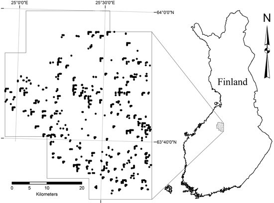
Fig. 1. ALS data coverage and sample plot location.
The field data of our study consisted of total 852 reference plots. The data of 799 plots were measured by the FFC to be used as reference data for stand-level forest inventory carried out using ABA in summer 2012. These plots were mainly allocated to productive forests, thus there was a lack of reference plots from low-productive forests. Therefore, 53 plots were measured in the field from poorly-growing forestry-drained peatlands in autumn 2013 to augment the field data.
Both the field sample design and the field measurements were performed according to the procedure used by the FFC (Heikkilä et al. 2011). The field data consisted of plots located in random clusters, where one cluster consisted of 6–9 circular sample plots with a radius of 9 m. One cluster was estimated to be equivalent to one day of field work. The predefined plot locations were positioned by a hand-held GPS device, and the locations were post-processed using virtual reference station data. Tree species and diameter at breast height (DBH) were measured from every tree with a DBH of at least 5 cm. Tree height and age were measured from at most three sample trees per species per plot: the basal area mean tree, one larger tree and one smaller tree.
Forest inventory attributes were computed for 799 plots during the FFC field campaign using tree height and stem volume models based on national forest inventory (NFI) data. Tree heights of the additional 53 plots were estimated according to height models of Veltheim (1987) and calibrated to the plot -level using sample tree data. Stem volumes were next estimated according to the species-specific stem volume models of Laasasenaho (1982). In summary, we had highly equivalent field data from two separate field campaigns.
2.2 ALS data
ALS data covering our study area were acquired by the National Land Survey of Finland (NLS). The data were collected during leaf-off canopy conditions on May 19–21, 2012, using a Leica ALS50 SN069 laser scanner. Flying altitude was 2200 m above ground level, with a pulse density of 0.8 pulses per m2, and the data included information from the first and the last echoes. The pre-processed data are freely available from the NLS (2015).
The digital terrain model (DTM) was produced from the last pulse data with TerraScan software (see www.terrasolid.fi) using the triangulation method explained in Axelsson (2000). Ground height was then subtracted from the laser pulse heights to produce a point cloud with XY -coordinates and the height above ground. Finally, 38 predictor variables (Table 1) were extracted to the reference plots from the height distribution of ALS points.
| Table 1. Predictor candidates (n = 38) derived from ALS data. | |
| Variable name | Variable description |
| h10f – h100f | Point height at the r percentile of the first-echo points’ height distribution (r = 10, 20... 100); ground points, i.e. points below the ground threshold (= 2 m), are excluded. |
| h10l – h100l | Point height at the r percentile of the last-echo points’ height distribution (r = 10, 20... 100); ground points are excluded. |
| penef | Penetration of first-echo points; calculated as the ratio of the number of ground points to the number of all points |
| penel | Penetration of last-echo points |
| HVmean | The mean of the first-echo high-vegetation points, i.e. points above the high vegetation threshold (= 5 m) |
| HVsd | Standard deviation of the Z coordinates for the high vegetation first-echo points |
| pc1l – pc8l | Ratio of the number of last-echo points with heights smaller or equal to hmax to the number of all last-echo points, where hmax = hclassstart + i * hclasssize (i = 1, 2… 8; hclassstart = 1.5 m; hclasssize = 2.0 m) |
| p8530f | Proportional canopy density at a height equalling 30% of the 85th percentile of first-echo points’ height distribution; calculated as the ratio of the number of first-echo points below that height to the number of all first-echo points |
| p8580f | Proportional canopy density at a height equalling 80% of the 85th percentile of first-echo points’ height distribution |
| p9030f | Proportional canopy density at a height equalling 30% of the 90th percentile of first-echo points’ height distribution |
| p9080f | Proportional canopy density at a height equalling 80% of the 90th percentile of first-echo points’ height distribution |
| p9530f | Proportional canopy density at a height equalling 30% of the 95th percentile of first-echo points’ height distribution |
| p9580f | Proportional canopy density at a height equalling 80% of the 95th percentile of first-echo points’ height distribution |
3 Methods
3.1 General workflow of the study
The aim of the analysis was to study 1) the accuracy of ABA in predicting forest inventory attributes for forests growing on LPDPs and 2) how the number of reference plots measured from LPDPs in addition to 500 plots measured from productive forests effects the k-NN prediction accuracy. We also investigated how reference plots allocated to LPDPs affected the prediction accuracy of forest inventory attributes in productive forests. We used the following workflow in our analysis (illustrated in Fig. 2):
- All the reference plots from forestry-drained peatlands were classified as either productive or low-productive forests (see section 3.2).
- The subset of 500 plots from productive forests and the subsets of 0, 5, 10, …, 50 and 58 LPDP plots were generated using two ALS-derived metrics that correlated well with Lorey’s height (h80f,) and basal area (penef,). Thus, it was ensured that field data variation was maintained in the subsets as well as possible.
- The strongest predictor variables for stem volume (V), stem number (N), mean diameter (dg) and proportion of deciduous trees (deciduous%) were searched separately and selected for further analyses. Then, the strongest predictors of V, N, dg and deciduous% were searched simultaneously and selected for forest inventory attribute prediction. The variable selection was carried out using reference data consisting of 500 plots from productive forests and 58 plots from LPDPs (see section 3.3.1).
- Forest inventory attributes were predicted using the reference data and the random forests (RF) technique in k nearest neighbour (k-NN) mode (see section 3.3.2).
- Prediction accuracy was validated separately for LPDPs, young productive stands and mature stands using leave-one-out cross validation. The sensitivity of predictions to the number of additional LPDP reference plots was evaluated by iteratively adding more LPDP plots to the reference data and repeating step 4 until all LPDP plots were used in the estimation (see section 3.4).
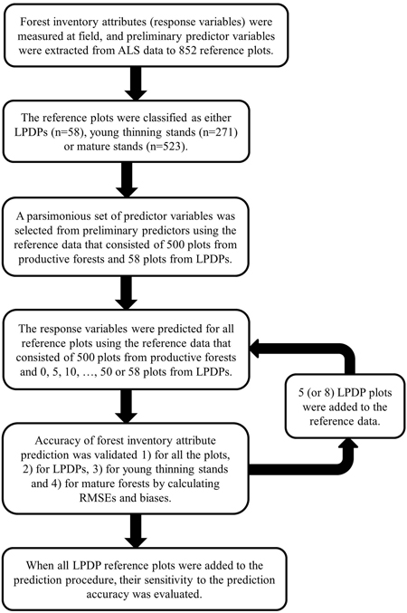
Fig. 2. General workflow of the analysis.
3.2 Classification of productive and low-productive forestry-drained peatlands
In Finland, forest productivity is defined according to the average annual stem volume growth during the forest rotation period. The volume growth of productive forests is at least 1 m3 ha–1 per year, while the growth of poorly productive forests is 0.1–1 m3 ha–1 per year and less than that on unproductive forests. In our study, all the forests growing less than 1 m3 ha–1 per year were classified as low-productive forests.
The productive and low-productive forestry-drained peatlands were classified based on total stem volume, stem number and basal area (G). Forest management experts at Metsähallitus (the Finnish state-owned forest enterprise) have defined the minimum basal area as 6 m2 ha–1 and the minimum stem number as 650 stems per hectare for productive peatlands drained 30–50 years ago. We also set the maximum level for stem volume in LPDPs to 60 m3 ha–1 because otherwise some productive stands would have been misclassified due to low stem number. In summary, drained peatlands were classified as productive if G ≥ 6 m2 ha–1 and N ≥ 650 ha–1 or V ≥ 60 m3 ha–1.
3.3 k-NN prediction of forest inventory attributes using random forests
The k-NN estimation technique is a common approach for predicting multiple species-specific forest inventory attributes from remote sensing data (e.g. Poso 1972; Tomppo 1990). Here, the objective was to predict forest inventory data (response variables) using remotely-sensed auxiliary data (predictor variables). The predictions were based on reference data where both the response and predictor variables were available. In ABA, forest inventory data are predicted for grid cells (usually 16 m x 16 m in Finnish forest inventory) by searching the k nearest reference plots for every grid cell across the entire inventory area and calculating the response variables as a weighted mean over those neighbours.
Several methods are available for selecting “nearest neighbours” from the reference data. In our study, the neighbours were selected using the RF technique developed by Breiman (2001) because it has been reported as a robust and flexible method compared to many other k-NN methods (Hudak et al. 2008; Latifi and Koch 2012). The RF technique is based on several classification trees generated from random subsets of predictor variables. The similarity of target and reference observations is defined according to their probability of ending up in the same terminal node after RF classification; high proximity means small statistical distance and vice versa. The k-NN prediction of forest inventory attributes using RF is explained in detail in Crookston and Finley (2008), Hudak et al. (2008), Falkowski et al. (2010) and Yu et al. (2011).
3.3.1 Predictor variable reduction
Prior to k-NN predictions, the number of predictor variables must be reduced to obtain a parsimonious subset of predictors (Hudak et al. 2008). We used RF iterations in the sequential backward feature selection method for reducing the number of predictors. At first, we searched the most important predictors separately for four response variables (V, N, dg and deciduous%). The procedure began with 38 preliminary predictor variables; in each iteration round the least important predictor was discarded based on variable importance until the five most important predictors remained. To do this, we used the yaiVarImp function of the yaImpute package in statistical software (see www.r-project.org) developed by Crookston and Finley (2008). Due to randomness of the RF technique, the procedure was repeated 200 times for each response variable, and the predictors matching the five best predictors at least 100 times were saved for further testing. The best predictors of stem volume (penef, h50f, pc5l, h70f, p9530f), stem number (HVsd, penef, h20l, p9030f), mean diameter (h100f, h80l, h90l, h90f) and proportion of deciduous trees (HVsd, pc4l, h30l, pc2l) were combined to one variable set and, after removing the duplicates, we ended up with a subset of 15 candidate predictors (see Fig. 3).
The final predictor variable selection was performed using the varSelection function of the yaImpute package in R software. The backward feature selection algorithm began with all candidate predictors and deleted them one at a time by computing the mean Mahalanobis distance between the observed and estimated values of V, N, dg and deciduous%. So, the function calculated which predictor could be removed from the predictor set by weakening the prediction accuracy the least, thus the predictor related to the largest Mahalanobis distance was discarded in every iteration round. The entire variable selection procedure was repeated 100 times, and variables that were selected by the function at least every third time and that had less than 0.9 correlation with all the other selected variables were used to predict forest inventory attributes. The maximum correlation between two predictors was limited to 0.9 similarly as in Hudak et al. (2008) aiming to restrict undue redundancy.
3.3.2 Forest inventory attribute prediction
Total stem volume, stem number, mean diameter and proportion of deciduous trees were selected as dependent response variables for the prediction because V, N and dg are important harvesting cost indicators (Laitila 2008) and deciduous% explains tree species composition. Basal area and Lorey’s height (hg) were also predicted, but they were not used as dependent variables due to their strong correlations with V and dg, respectively. In our study, 250 classification trees were generated for every dependent response variable, thus we had a total of 1000 classification trees, where all four dependent response variables had an equal importance. The square root of the number of predictors was randomly picked for the nodes of each classification tree.
Parameter k was varied from 1 to 10 and finally set at 3 because this resulted in the lowest RMSE of stem volume estimates in LPDPs while only a small number of LPDP reference plots were used in the prediction. Tuominen et al. (2003) tested k values from 3 to 5 and concluded that within this range a k value increase would improve estimation accuracy but concurrently diminish the variation retained in the estimates.
3.4 Accuracy evaluations
Forest inventory attribute estimates were validated using leave-one-out cross validation at 254 m2 resolution. The prediction was repeated 25 times, and the final results were computed as the mean values of the iterations. Estimation accuracy was evaluated by calculating bias and RMSE (Eq. 1 and Eq. 2, respectively).

 where n was the number of plots, yi was the observed value for plot i and ŷi was the predicted value for plot i. The relative bias and RMSE were calculated in relation to the observed mean of the variable in question.
 Extrapolating forest inventory attributes outside the field data range is impossible when the k-NN estimation method is used, thus reference data are always required from each stand type for which forest inventory is being applied. The requirement of the field-measured LPDP reference plots and their effect on prediction accuracy were evaluated by iteratively adding LPDP plots to the reference data. Initially, the reference data consisted of 500 plots from productive forests only, imitating the typical reference data used in ABA forest inventory by the FFC. Next, five LPDP plots at a time were added to the reference data, and the procedure was repeated until all LPDP plots were used in the prediction.
Prediction accuracy was validated after each iteration round 1) for all the plots, 2) for LPDPs, 3) for productive young thinning stands and 4) for productive advanced-thinning and mature stands (see the descriptions of stand development classes in Table 2). The stand development classes were defined by FFC forest professionals during the field measurements. Productive forests were divided into these two evaluation classes because the extra LPDP reference plots might presumably have an effect on forest attribute estimates especially in young, thinning stands. The statistics about the classes used in the evaluation are presented in Table 3.
| Table 2. Stand development classes on productive forest land. The classification system and the terminology follow the Finnish Forest Research Institute (2014). | |
| Development class | Definition |
| Young thinning stand | The stands are at a developmental stage where harvesting mostly produces pulpwood. Mean stem DBH is 8–16 cm. |
| Advanced thinning stand | The stands are at a developmental stage and the next forest operation is thinning. Most stems are of saw-timber size, as mean stem DBH is more than 16 cm. |
| Mature stand | The stands are mature and the most profitable forest operation is regeneration cutting. The lower limit for mean stem DBH varies from 23 cm to 29 cm according to location, soil quality and tree species. |
| Table 3. Summary of the reference plot data. | |||
| Forest inventory attribute | Range | Mean | SD |
| Low-productive drained peatlands (n = 58) | |||
| hg, m | 3.8–19.0 | 8.6 | 3.2 |
| dg, cm | 5.5–19.9 | 10.9 | 3.5 |
| N, ha–1 | 79–1690 | 547 | 332 |
| G, m2 ha–1 | 0.2–8.3 | 3.7 | 2.1 |
| V, m3 ha–1 | 0.5–58.7 | 18.7 | 14.2 |
| T, years | 25–122 | 50 | 16 |
| Tree species proportion of total basal area | |||
| Pine (%) | 0–100 | 64 | 44 |
| Spruce (%) | 0–100 | 5 | 19 |
| Deciduous (%) | 0–100 | 31 | 41 |
| Young thinning stands (n = 271) | |||
| hg, m | 6.0–17.7 | 10.6 | 2.1 |
| dg, cm | 7.3–22.8 | 12.3 | 2.5 |
| N, ha–1 | 275–7270 | 1996 | 1071 |
| G, m2 ha–1 | 2.1–29.2 | 14.0 | 5.4 |
| V, m3 ha–1 | 10.6–212.8 | 77.8 | 37.6 |
| T, years | 15–114 | 42 | 18 |
| Tree species proportion of total basal area | |||
| Pine (%) | 0–100 | 57 | 40 |
| Spruce (%) | 0–100 | 17 | 27 |
| Deciduous (%) | 0–100 | 26 | 30 |
| Advanced thinning and mature stands (n = 523) | |||
| hg, m | 10.0–27.8 | 16.9 | 3.0 |
| dg, cm | 11.8–45.0 | 20.5 | 4.6 |
| N, ha–1 | 196–3615 | 1099 | 569 |
| G, m2 ha–1 | 4.6–50.9 | 21.9 | 8.0 |
| V, m3 ha–1 | 32.7–499.2 | 181.9 | 85.7 |
| T, years | 26–153 | 74 | 21 |
| Tree species proportion of total basal area | |||
| Pine (%) | 0–100 | 52 | 38 |
| Spruce (%) | 0–100 | 29 | 34 |
| Deciduous (%) | 0–100 | 19 | 24 |
4 Results
4.1 Selected predictor variables
The importance of 15 candidate predictors in the k-NN forest inventory attribute prediction is illustrated in Fig. 3. Variables h70f, h30l, h80l and p9530f were chosen for the prediction according to the criteria defined in section 3.3.1. Variable h70f correlated highly with Lorey’s height (0.98 correlation in all field plots and 0.96 in LPDPs), and it was the most important predictor for forest canopy height. Variable p9530f was sensitive to the variation in vegetation density as the variable correlates well with basal area (correlations of 0.79 and 0.61 in all field plots and in LPDPs, respectively. The predictors related to proportional canopy density discriminated low-productive and productive forests rather well, as average p9530f value was clearly lower in LPDPs (0.21) than in thinning and mature forests (0.56 and 0.61, respectively). Variable h30l was an important predictor due to its sensitivity to deciduous% (–0.43 correlation) and its low correlations with other selected predictors.
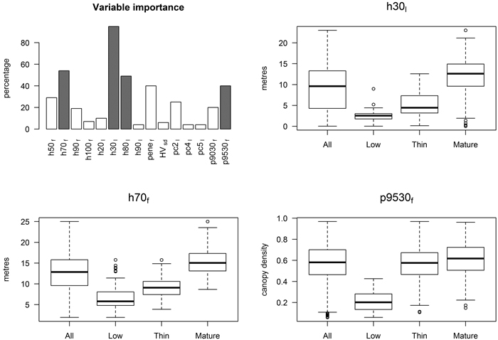
Fig. 3. The importance of 15 candidate predictors (the selected predictors are grey -coloured) and the variation of three selected predictors in LPDPs, thinning and mature forests.
4.2 Accuracy of forest inventory attribute prediction
The prediction accuracy of Lorey’s height, mean diameter, stem number, basal area and stem volume was analysed with varying number of LPDP plots in the reference data (Fig. 4). Following current forest inventory practises and having only 500 plots measured from productive forest stands in the reference data, the RMSEs (and relative RMSEs) for the prediction accuracies were 1.4 m (16%), 2.1 cm (19%), 700 ha–1 (128%), 2.7 m2 ha–1 (72%) and 13.7 m3 ha–1 (73%) in LPDPs, respectively. When 30 reference plots from LPDPs were added to the k-NN estimation (allocation is presented in Fig. 5), the respective accuracies were improved to 1.1 m (13%), 2.1 cm (20%), 360 ha–1 (65%), 1.7 m2 ha–1 (46%) and 10.0 m3 ha–1 (53%). Only minor improvement was observed in the predictions when more than 30 LPDP plots were added to the reference data (see Fig. 4).
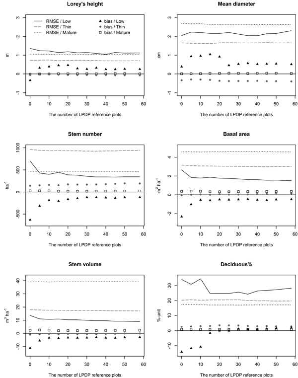
Fig. 4. Estimation accuracy of forest inventory attributes with a varying number of reference plots from LPDPs used in the prediction.
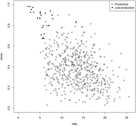
Fig. 5. Allocation of 500 reference plots on productive forest stands and 30 reference plots on LPDPs according to two features extracted from ALS data.
LPDPs are mainly dominated by either pine (Pinus sylvestris) or downy birch (Betula pubescens ssp. pubescens). Having 30 LPDP plots in the reference data, plot-level stem volume was predicted with RMSEs of 8.9 m3 ha–1 and 12.4 m3 ha–1 in pine- (n = 37) and birch-dominated (n = 18) LPDPs, respectively (Table 4). Overall, the proportion of deciduous trees was predicted with 26%-units of RMSE. However, the main tree species was predicted with 87% accuracy in LPDP reference plots, which means that pine- and birch-dominated stands can be discriminated reasonably well by ABA.
| Table 4. Estimation accuracy of pine- and birch-dominated LPDPs when 30 reference plots from LPDPs were added to the reference data. | ||||
| RMSE | RMSE % | Bias | Bias % | |
| Pine-dominated LPDPs (n = 37) | ||||
| hg, m | 1.0 | 13 | 0.2 | 2.1 |
| dg, cm | 2.1 | 21 | 0.4 | 4.4 |
| N, ha–1 | 298 | 60 | –116 | –23 |
| G, m2 ha–1 | 1.5 | 46 | –0.4 | –12 |
| V, m3 ha–1 | 8.9 | 59 | –2.3 | –15 |
| Birch-dominated LPDPs (n = 18) | ||||
| hg, m | 1.4 | 13 | 0.4 | 4.1 |
| dg, cm | 1.9 | 16 | 0.5 | 4.4 |
| N, ha–1 | 377 | 63 | –133 | –22 |
| G, m2 ha–1 | 2.1 | 46 | –0.7 | –15 |
| V, m3 ha–1 | 12.4 | 49 | –5.2 | –21 |
Additional reference data allocation did not affect the forest inventory attribute predictions in productive forest stands. Regardless of the number of LPDP plots in the k-NN estimation, hg, dg, N, G and V were predicted for young productive stands in the developmental stage with the following relative RMSEs: 7%, 13%, 46%, 22% and 22%.
5 Discussion
The aim of the study was to evaluate the suitability of ABA for mapping the forest inventory attributes in forests growing on LPDPs. Due to the updated forest legislation this is a current topic in several Finnish forest companies (e.g. Metsähallitus). Metsähallitus manages 35% of the forestry land in Finland, and the majority of its forest holdings are located in Northern Finland. It administers a total 272 000 hectares of LPDPs, according to its forest management geographic information system. The forest managers of Metsähallitus are updating their forest inventory data and planning the management of their LPDPs. Practically no cuttings have been performed in LPDPs due to the old forest legislation because harvesting low timber volumes, maintaining ditch networks and cultivating new forest generations would have been unprofitable. Therefore, the renewed legislation released more exploitable wood biomass resources, especially in Northern Finland, and Metsähallitus would like to test the suitability of ALS to map potential LPDPs for bioenergy harvesting and to update forest inventory data for the cost accounting of wood procurement. An aerial photograph and mapped stem volume of the study area are presented in Fig. 6. A potential area for biomass harvesting without the forest regeneration prerequisite is located in the southwest corner of the map.
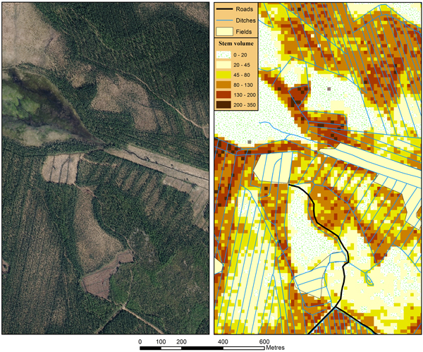
Fig. 6. An aerial photograph (© NLS 2014) and mapped stem volume (m3 ha–1) of the study area.
The restoration of ecosystems is an important tool for maintaining ecosystem services and restraining biodiversity loss, thus Metsähallitus attempts to restore some peatland ecosystems that have been degraded by drainage campaigns. LPDPs are good targets for restoration because they have a low significance for forestry and, in natural conditions, offer important habitats for grouses. The main ecological objectives of peatland restoration are to re-establish peatlands’ hydrological features close to natural conditions and to trigger ecological succession that will lead to the near-natural functioning of peatland ecosystems (Similä et. al. 2014). In their current state, nutrient-poor, forestry-drained peatlands are CO2 sinks that have a cooling impact on the climate (Ojanen et al. 2012). Restoration of forestry-drained peatlands involves raising water tables, which increases these CO2 sinks (Soini et al. 2010), but otherwise restoration also has a warming impact on the climate as CH4 emissions increase (Juottonen et al. 2012). The long-term climate impacts of restoring forestry-drained peatlands are being monitored, and more data are needed before we can make any further conclusions.
We used ALS data collected by the NLS, which produces a national digital terrain model (DTM) using low-pulse-density ALS data acquired during leaf-off canopy conditions. Leaf-off ALS data are favoured in DTM modelling because understory vegetation causes serious bias in the DTMs produced from ALS data acquired in leaf-on conditions (Sirkiä and Laaksonen 2009). Forest inventory and mapping applications have been studied mainly using leaf-on ALS data, but we used the same leaf-off ALS data as the NLS used for the DTM modelling because the multiple uses of data would mean significant cost savings for both DTM production and forestry applications. Næsset (2005) suggested that canopy conditions affect the last echoes more than the first echoes of laser pulses, and the height distribution of the returns is more diverse during leaf-off than leaf-on conditions. In previous studies, ABA prediction accuracy for both total and species-specific stem volumes has been approximately equal using either leaf-off or leaf-on ALS data (Næsset 2005; Villikka et al. 2012). Villikka et al. (2012) concluded that leaf-off ALS data are suitable for forest inventory, but data collection is restricted because the leaf-off season without snow is short in the Nordic climate. It should be noted that the use of leaf-off data has not been a common practice in forest inventory (White et al. 2013), though currently leaf-off data is often used because ALS-based DTM modelling is underway in Finland and in many other countries.
The accuracy of predictions obtained by ABA was in line with previous studies when comparing prediction accuracies in thinning and mature stands. Reference plots from LPDPs did not affect the accuracy of forest inventory attribute prediction in productive forest stands. For Lorey’s height, mean diameter, stem number, basal area and stem volume we obtained the respective relative RMSEs of 7%, 13%, 46%, 22% and 22% in young thinning stands, and 6%, 13%, 42%, 21% and 22% in mature plots. Previously the accuracies have varied, respectively, between 6–10%, 13–20%, 25–50%, 14–23% and 17–23% (e.g. Næsset et al. 2004; Maltamo et al. 2006; Vastaranta et al. 2013).
Forest inventory attributes of LPDPs were successfully predicted using low-pulse-density ALS data. To our knowledge, the most similar study to ours was presented by Nyström et al. (2012). Using corresponding ALS data to map mountain birch biomass in the forest-tundra ecotone, they reported 9.5%, 21.2% and 18.7% relative RMSEs for the plot-level estimation accuracies of maximum tree height, AGB and vertical canopy cover, respectively. The relative errors of biomass or stem volume estimates were larger in our study, but in our study area the growing stocks were smaller and more heterogeneous, including more diverse habitats and a few different tree species.
Without any LPDP plots in the reference data, the k-NN method gives inaccurate and biased estimates for LPDPs. In our study area the prediction accuracy improved quickly when some LPDP plots were added to the prediction, but only minor improvement was observed after having approximately 30 LPDP reference plots in addition to the 500 plots measured from productive forests in the reference data (Fig. 4). The RMSE of total stem volume estimates was improved 27% when the number of LPDP reference plots was increased from 0to 30, but the respective improvement was only 9% when the number was increased from 30 to 58.
Sampling of the LPDP reference plots could be performed using two ALS-derived metrics i.e., one feature correlating with mean tree height and another correlating with basal area (h80f and penef were used in our study). The expansion of the reference data in relation to these two variables is presented in Fig. 5. Often, the scale of forest inventory attributes is close to one another in LPDPs and young productive forests, but the figure illustrates that these forest types could be discriminated well by ALS.
If ABA is applied out of the typical range of forest conditions, it should be taken into account. There are many areas around the world similar to boreal LPDPs where ALS forest inventory could be applied (e.g. coastal or mountainous forests). The prediction accuracy and the required reference data are always case -specific, but our study showed that the results can be improved by measuring a few plots from the new strata. Our methodology can be applied for optimising the campaign-specific requirement of reference data from different stratums in relation to inventory costs and benefits.
6 Conclusions
We applied ALS-based ABA forest inventory for naturally sparse growing stocks that have not been generally inventoried. The reference plot data were acquired from Haapajärvi, which imitated well the typical field data sample collected for ABA in Finland. There were no plots measured from LPDPs, thus we measured additional reference plots from this stratum to apply ABA to those areas.
The overall conclusion is that ABA is a suitable method for predicting forest inventory attributes in poorly productive boreal forests if reference plots are allocated to this stratum. When reference plots are allocated only for productive forests, predictions in forests growing on LPDPs are biased. If reference plots are measured from LPDPs, ABA can be used for biomass mapping and for forest management planning (e.g. harvesting cost assessment) in those areas.
Acknowledgements
This research was commissioned by Metsähallitus and it was made possible by financial aid from Tekes project “Sustainable Bioenergy Solution for Tomorrow” (BEST) and the Academy of Finland project “Centre of Excellence in Laser Scanning Research” (CoE-LaSR). We also want to thank Nuutti Kiljunen and Paavo Soikkeli from Metsähallitus and the anonymous reviewers for their valuable comments and suggestions.
References
Axelsson P. (2000). DEM generation from laser scanner data using adaptive TIN models. In: International Archives of Photogrammetry and Remote Sensing, Amsterdam 33(B4): 110–117.
Breiman L. (2001). Random forests. Machine Learning 45(1): 5–32.
Crookston N.L., Finley A.O. (2008). yaImpute: an R package for kNN imputation. Journal of Statistical Software 23(10): 1–16.
Falkowski M.J., Hudak A.T., Crookston N.L., Gessler P.E., Uebler E.H., Smith A.M.S. (2010). Landscape-scale parameterization of a tree-level forest growth model: a k-nearest neighbor imputation approach incorporating LiDAR data. Canadian Journal of Forest Research 40(2): 184–199. http://dx.doi.org/10.1139/X09-183.
Finnish Forest Research Institute (2014). Finnish statistical yearbook of forestry. 428 p. ISBN 978-951-40-2506-8.
Heikkilä J., Ärölä E., Kilpiäinen S. (2011). Kaukokartoitusperusteisen metsien inventoinnin koealojen maastotyöohje (versio 1.1). 23 p. [In Finnish].
Hudak A.T., Crookston N.L., Evans J.S., Hall D.E., Falkowski M.J. (2008). Nearest neighbor imputation of species-level, plot-scale forest structure attributes from LiDAR data. Remote Sensing of Environment 112(5): 2232–2245. http://dx.doi.org/10.1016/j.rse.2007.10.009.
Hyyppä J., Hyyppä H., Leckie D., Gougeon F., Yu X., Maltamo M. (2008). Review of methods of small-footprint airborne laser scanning for extracting forest inventory data in boreal forests. International Journal of Remote Sensing 29(5): 1339–1366. http://dx.doi.org/10.1080/01431160701736489.
Juottonen H., Hynninen A., Nieminen M., Tuomivirta T.T., Tuittila E.-S., Nousiainen H., Kell D.K., Yrjälä K., Tervahauta A., Fritze H. (2012). Methane-cycling microbial communities and methane emission in natural and restored peatlands. Applied Environmental Microbiology 78(17): 6386–6389. http://dx.doi.org/10.1128/AEM.00261-12.
Laasasenaho J. (1982). Taper curve and volume functions for pine, spruce and birch. Communicationes Instituti Forestalis Fenniae 108. 74 p.
Laitila J. (2008). Harvesting technology and the cost of fuel chips from early thinnings. Silva Fennica 42(2): 267–283. http://dx.doi.org/10.14214/sf.256.
Latifi H., Koch B. (2012). Evaluation of most similar neighbour and random forest methods for imputing forest inventory variables using data from target and auxiliary stands. International Journal of Remote Sensing 33(21): 6668–6694. http://dx.doi.org/10.1080/01431161.2012.693969.
Maltamo M., Malinen J., Packalén P., Suvanto A., Kangas J. (2006). Nonparametric estimation of stem volume using airborne laser scanning, aerial photography, and stand-register data. Canadian Journal of Forest Research 36: 426–436. http://dx.doi.org/10.1139/X05-246.
Maltamo M., Bollandsås O.M., Næsset E., Gobakken T., Packalén P. (2011a). Different plot selection strategies for field training data in ALS-assisted forest inventory. Forestry 84(1): 23–31. http://dx.doi.org/10.1093/forestry/cpq039.
Maltamo M., Packalén P., Kallio E., Kangas J., Uuttera J., Heikkilä J. (2011b). Airborne laser scanning based stand level management inventory in Finland. Proceedings of SilviLaser 2011, 11th International Conference on LiDAR Applications for Assessing Forest Ecosystems, University of Tasmania, Australia, 16–20 October 2011. p. 1–10.
Næsset E. (2002). Predicting forest stand characteristics with airborne scanning laser using a practical two-stage procedure and field data. Remote Sensing of Environment 80(1): 88–99. http://dx.doi.org/10.1016/S0034-4257(01)00290-5.
Næsset E. (2005). Assessing sensor effects and effects of leaf-off and leaf-on canopy conditions on biophysical stand properties derived from small-footprint airborne laser data. Remote Sensing of Environment 98(2–3): 356–370. http://dx.doi.org/10.1016/j.rse.2005.07.012.
Næsset E., Gobakken T., Holmgren J., Hyyppä H., Hyyppä J., Maltamo M., Nilsson M., Olsson H., Persson Å., Söderman U. (2004). Laser scanning of forest resources: the Nordic experience. Scandinavian Journal of Forest Research 19(6): 482–499. http://dx.doi.org/10.1080/02827580410019553.
National Land Survey of Finland (2015). Datasets free of charge. http://www.maanmittauslaitos.fi/en/opendata. [Cited 5 Feb 2015].
Natural Resources Institute Finland (2015). LIFEPeatLandUse: quantification and valuation of ecosystem services to optimize sustainable re-use for low-productive drained peatlands. http://www.metla.fi/hanke/8547/index-en.htm. [Cited 5 Feb 2015].
Nyström M., Holmgren J., Olsson H. (2012). Prediction of tree biomass in the forest-tundra ecotone using airborne laser scanning. Remote Sensing of Environment 123: 271–279. http://dx.doi.org/10.1016/j.rse.2012.03.008.
Ojanen P., Minkkinen K., Penttilä T. (2012). The current greenhouse gas impact of forestry-drained boreal peatlands. Forest Ecology and Management 289: 201–208. http://dx.doi.org/10.1016/j.foreco.2012.10.008.
Paavilainen E., Päivänen J. (1995). Peatland forestry: ecology and principles. Springer, Berlin. 248 p. ISBN 978-3-540-58252-6.
Poso S. (1972). A method of combining photo and field samples in forest inventory. Communicationes Instituti Forestalis Fenniae 76(1). 133 p.
Similä M., Aapala K., Penttinen J. (2014). Ecological restoration in drained peatlands – best practices from Finland. Metsähallitus, Natural Heritage Services, Vantaa. ISBN 978-952-295-072-7.
Sirkiä O., Laaksonen H. (2009). Kesäkeilausten soveltuvuudesta korkeusmallituotantoon. Kevätlaser metsävarojen inventoinnissa. MMM:n konserniohjelmahankkeen loppuraportti (proj. n:o 311100). [Final report, in Finnish].
Soini P., Riutta T., Yli-Petäys M., Vasander H. (2010). Comparison of vegetation and CO2 dynamics between a restored cut-away peatland and a pristine fen: evaluation of the restoration success. Restoration Ecology 18(6): 894–903. http://dx.doi.org/10.1111/j.1526-100X.2009.00520.x.
Tomppo E. (1990). Satellite image-based national forest inventory of Finland. The Photogrammetric Journal of Finland 12(1): 115–119.
Tuominen S., Fish S., Poso S. (2003). Combining remote sensing, data from earlier inventories, and geostatistical interpolation in multisource forest inventory. Canadian Journal of Forest Research 33(4): 624–634. http://dx.doi.org/10.1139/x02-199.
Vastaranta M., Wulder M.A., White J.C., Pekkarinen A., Tuominen S., Ginzler C., Kankare V., Holopainen M., Hyyppä J., Hyyppä H. (2013). Airborne laser scanning and digital stereo imagery measures of forest structure: comparative results and implications to forest mapping and inventory update. Canadian Journal of Remote Sensing 39(5): 382–395. http://dx.doi.org/10.5589/m13-046.
Veltheim T. (1987). Pituusmallit männylle, kuuselle ja koivulle. M.Sc. thesis, Faculty of Agriculture and Forestry, University of Helsinki, Finland. [In Finnish].
Villikka M., Packalén P., Maltamo M. (2012). The suitability of leaf-off airborne laser scanning data in an area-based forest inventory of coniferous and deciduous trees. Silva Fennica 46(1): 99–110. http://dx.doi.org/10.14214/sf.68.
White J.C., Wulder M.A., Varhola A., Vastaranta M., Coops N.C., Cook B.D., Pitt D, Woods M. (2013). A best practices guide for generating forest inventory attributes from airborne laser scanning data using the area-based approach. Information Report FI-X-10. Natural Resources Canada, Canadian Forest Service, Canadian Wood Fibre Centre, Victoria, BC. 50 p.
Wulder M.A., Coops N.C., Hudak A.T., Morsdorf F., Nelson R., Newnham G., Vastaranta M. (2013). Status and prospects for LiDAR remote sensing of forested ecosystems. Canadian Journal of Remote Sensing 39 (supplement 1): S1–S5. http://dx.doi.org/10.5589/m13-051.
Yu X., Hyyppä J., Vastaranta M., Holopainen M., Viitala R. (2011). Predicting individual tree attributes from airborne laser point clouds based on the random forests technique. ISPRS Journal of Photogrammetry and Remote Sensing 66(1): 28–37. http://dx.doi.org/10.1016/j.isprsjprs.2010.08.003.
Total of 35 references
