Jena Ferrarese  ,
David Affleck,
Carl Seielstad
,
David Affleck,
Carl Seielstad
Conifer crown profile models from terrestrial laser scanning
Ferrarese J., Affleck D., Seielstad C. (2015). Conifer crown profile models from terrestrial laser scanning. Silva Fennica vol. 49 no. 1 article id 1106. https://doi.org/10.14214/sf.1106
Highlights
- Crown models are derived from terrestrial laser data for 3 NW USA conifer species
- Crown models require only crown length for implementation
- Beta and Weibull curves fit to 95th percentile widths describe crown extent
- Crown profile curves are species-specific and not interchangeable
- Crown shape is not strongly conditioned by tree size or site.
Abstract
Regional crown profile models were derived for three conifer species of the interior northwestern USA from terrestrial laser scans of eighty-six trees across a range of sizes and growing conditions. Equations were developed to predict crown shape from crown length for Pseudotsuga menziesii, Pinus ponderosa, and Abies lasiocarpa from parametric curves applied to crown-length normalized laser point clouds. The 95th width percentile adequately described each crown’s outer limit; alternate width percentiles produced little profile shape variation. For P. menziesii and P. ponderosa, a scaling parameter-modified beta curve gave the most accurate fit (using cross-validated Mean Absolute Error) to aggregated 95th width percentile points. For A. lasiocarpa, beta and Weibull curves (equivalently modified) produced similar results. For all species, modified beta and Weibull curves fit crown points with less error than conic or cylindrical profiles. Crown profile curves were species-specific; interchanging among species increased error significantly. Laser-derived crown base metrics provided objectivity and consistency, but underestimated field-derived base heights through inclusion of dead branches. Profile curve parameters were not correlated with tree or stand characteristics suggesting that crown shape is not strongly conditioned by size and site factors. However, laser sampling necessarily favored more open growing conditions, potentially under-representing variations in crown shape associated with social position. Overall, Terrrestrial Laser Scanning (TLS) lends itself to detailed measurements of external crown architecture with occlusion-imposed limits to characterization of internal features. Yet, the time and cost of collecting and processing individual tree data precludes use of TLS as a common field sampling tool.
Keywords
prediction;
canopy shape;
parametric curves;
interior Northwest USA
-
Ferrarese,
College of Forestry and Conservation, The University of Montana, Missoula, MT, USA; (present) Center for the Environmental Management of Military Lands, 1490 Campus Delivery, Colorado State University, Fort Collins, CO 80523, USA
E-mail
jena.ferrarese@colostate.edu
- Affleck, College of Forestry and Conservation, University of Montana, Missoula, MT, USA E-mail david.affleck@cfc.umt.edu
- Seielstad, College of Forestry and Conservation, University of Montana, Missoula, MT, USA E-mail carl.seielstad@firecenter.umt.edu
Received 16 February 2014 Accepted 24 September 2014 Published 3 February 2015
Views 188813
Available at https://doi.org/10.14214/sf.1106 | Download PDF

1 Introduction
Understanding the distribution of the above-ground biomass of the dominant plants on landscapes is of critical and growing importance in forest conservation and management. Emerging interests in wildland fire behavior and risk (Hiers et al. 2009; Parsons et al. 2011; Ottmar et al. 2012), bioenergy utilization (Dassot et al. 2012; Fernandez-Sarria et al. 2013), carbon sequestration (Clark et al. 2011), and wildlife conservation (Lesak et al. 2011; Palminteri et al. 2012) among others, increasingly rely on accurate assessments of the amount and location of biomass, often at finer scales than traditional methods have provided. As field measurements are not always viable, scientists and managers employ models to infer biomass from tree lists, stand tables, and maps of vegetation composition and structure (Parresol 1999; Seidel et al. 2011). A conventional approach is to measure tree diameters and to estimate biomass from them using allometric equations derived from destructive sampling. Because most biomass allometries are necessarily constrained by small sample sizes and restricted geographic distributions, there is renewed effort to improve prediction effectiveness and reduce bias through application of more efficient sampling methods (Affleck and Turnquist 2012).
Beyond predicting the amount of biomass in forests and stands, there is considerable interest in understanding how biomass is distributed within individual tree crowns. The primary motivation driving the study of canopy architecture comes from the radiative transfer domain (Oker-blom and Kellomaki 1983; Duursma and Mäkelä 2007; Da Silva et al. 2008; Parveaud et al. 2008), but the arrangement of crown material is also important across a diverse array of interests ranging from long-established forest growth and competition modeling (Vanclay 1994) to novel approaches in wildland fire modeling that attempt to understand fire behavior and effects at very fine grains (Parsons et al. 2011; Hoffman 2012).
A logical approach to enumerate the spatial distribution of crown biomass is to quantify the space that the crown occupies, then to describe the internal heterogeneity of material, and, finally, to allocate biomass in a spatially-explicit manner, based on understanding of total biomass, crown volume and heterogeneity. In this research, we consider the initial step – deriving crown shape, using terrestrial laser scanning to collect detailed 3-dimensional data for many tree specimens and integrating the data to produce species-specific crown biomass envelopes for three common Rocky Mountain conifers. The research employs a novel approach for deriving crown shape (and hence volume) that is distinct from, but related to traditional crown profile modeling. We consider the spatial distribution of all laser returns from canopy materials in terms of height above ground and horizontal distance from bole centroids and produce volume and shape estimates from height and width percentiles.
The crown profile literature is robust, with direct and indirect modeling approaches described. Indirect methods begin by defining branch attributes (e.g., length and angle) and then computing crown envelopes from resulting trigonometric relationships (Cluzeau et al. 1994; Deleuze et al. 1996; Roeh and Maguire 1997). Direct methods utilize regression analysis to calculate crown width as a function of other, more easily measurable tree attributes such as total tree height, crown ratio or crown length, relative height within the crown or largest crown width (Biging and Wensel 1990; Baldwin and Peterson 1997; Hann 1999; Marshall et al. 2003; Crecente-Campo et al. 2009). Gill and Biging (2002) modeled crown profiles from photographs for five conifer species. Limitations of their approach to delineating crown profiles included photographic distortion, shading of crown edge, and visibility of, at most, two crown profiles per tree.
In contrast, Terrestrial Laser Scanning (TLS) provides essentially unlimited profiles per tree as data is captured from whole canopies, shading of crown edges is a non-issue presuming an unobstructed line of site exists, and distortion from photographic equipment and processing is not present. TLS is not without sources of error, however. For example, lower/front portions of a tree can partially or fully obscure the upper/back portions of the tree. Also, range error from diffuse targets and along hard edges can produce erroneous reflections in empty space, and wind can stir branch tips, resulting in multiple or missed measurements of crown elements. Nonetheless, with a sufficient number and density of pulses, many of the 3-D structural characteristics of a solid-with-interstices object (such as a tree crown) can be captured.
TLS has been used to characterize the vertical and horizontal patchiness within a tree crown and to quantify deviations from uniformity in arrangement of crown elements (Takeda et al. 2008). TLS has also been applied to studies of leaf area (Lovell et al. 2003; Henning and Radtke 2006; Beland et al. 2011; Sanz-Cortiella et al. 2011; Delagrange and Rochon 2011), gap fraction (Danson et al. 2007; Moorthy et al. 2008), radiative transfer (Côté et al. 2009), and canopy bulk density (Skowronski et al. 2011). In agricultural systems, laser scanning is viewed as one of the most promising techniques for capturing the geometry of tree crops (Rosell and Sanz 2012). Most recently, Fernandez-Sarria et al. (2013) used TLS to derive crown volumes of urban trees (using four different methods) and compared them with crown volumes derived from traditional field measurement techniques applied to three geometric volume models. TLS-derived volume estimates produced results consistent with traditional methods (R2 ≥ 0.78), but the research did not seek to define crown shape or to develop predictive models.
The overarching goal of this work is to develop species-specific models of crown shape and volume for common conifer species in the interior northwestern United States. To date, most TLS studies of forests have focused on detailed characterization of a limited number of trees or small plots (e.g. Henning and Radke 2006; Hosoi and Omasa 2006; Beland et al. 2011). Because our study intended to infer generalized crown shapes, a larger, more general sample was desired. This drove a sampling approach in which many trees of different sizes and growing conditions were each scanned from a single perspective rather than one or a few trees being scanned from many angles. Although limiting the information collected for any one tree, the approach produced data suitable for examining regional, species-level crown characteristics. Objectives of the study were fourfold: 1) To define an objective, repeatable crown base metric from TLS and assess differences in TLS-derived versus conventional field-measured crown base metrics; 2) To derive species-specific crown profile curves and compare differences among crown profile shapes and volumes using different crown-width percentiles; 3) To determine, through goodness-of-fit comparison, the best-fitting crown models for each species, and assess the accuracy of modeled curves relative to those resulting from simple geometric shapes (e.g., cones and cylinders); and 4) To examine species-specificity by assessing the fit between modeled curves of one species and crown profile points of another.
2 Methods
2.1 Study area
Data for three common Rocky Mountain conifer species (Pseudotsuga menziesii [Douglas-fir], Pinus ponderosa [ponderosa pine], and Abies lasiocarpa [subalpine fir]) were collected from 15 study sites in eastern Washington, northern Idaho and western Montana (Fig. 1 and Table 1). Stands were chosen to represent a variety of elevations, tree densities and site conditions; all sampling occurred in second-growth stands. P. menziesii and P. ponderosa were sampled in mixed conifer stands comprised of mixtures of P. menziesii, P. ponderosa, Pinus contorta, and Larix occidentalis. A. lasiocarpa was sampled in stands composed of A. lasiocarpa, Picea engelmannii, and Abies grandis. P. menziesii was sampled at elevations between 700–1850 m, P. ponderosa from 950–1850 m, and A. lasiocarpa from 1350–1900 m. Elevations and locations given in Table 1 were taken at the center of each selected stand; only one location point was taken regardless of the number of trees sampled at that site.
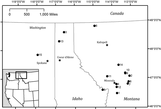
Fig. 1. Study sites across eastern WA, northern ID and western MT. Numeric labels correspond to site details in Table 1.
| Table 1. Study site information: name, sampled species, DBH range of sampled trees, basal area range as taken using the sample tree as plot center, and site elevation. Bracketed numbers indicate the number of each species sampled at each location. | ||||
| Site | Species sampled | DBH range (cm) | Basal area range (m2 ha–1) | Elevation (m) |
| 1. Ambrose Saddle | P. menziesii [3] P. ponderosa [1] A. lasiocarpa [6] | 49.4–60.0 63.6 11.5–62.7 | 9.2–16.1 2.3 34.4–68.9 | 1800 |
| 2. Bandy | P. menziesii [1] P. ponderosa [1] A. lasiocarpa [3] | 41.4 27.3 18.3–22.0 | 34.4 9.2 18.4–34.4 | 1350 |
| 3. Bonner’s Ferry | P. ponderosa [1] A. lasiocarpa [12] | 19.2 5.8–42.2 | 4.6 11.5–41.3 | 1500 |
| 4. Deer Creek | P. ponderosa [8] | 17.5–80.2 | 6.9–25.3 | 1300 |
| 5. Granite Pass | A. lasiocarpa [4] | 7.0–25.0 | not available | 1900 |
| 6. Kootenai | P. menziesii [4] P. ponderosa [4] | 16.4–30.2 17.4–62.9 | 6.9–18.4 9.2–36.7 | 1000 |
| 7. Lubrecht Garnet | P. menziesii [4] P. ponderosa [2] | 29.4–50.9 59.5–63.2 | 9.2–16.1 9.2–13.8 | 1850 |
| 8. Lubrecht Section 1 | A. lasiocarpa [1] | 14.2 | 9.2 | 1900 |
| 9. Lubrecht Stinkwater | A. lasiocarpa [1] | 37.0 | not available | 1550 |
| 10. Morrell Creek | P. menziesii [4] P. ponderosa [5] | 21.9–38.4 16.8–44.0 | 4.6–16.1 2.3–13.8 | 1350 |
| 11. Nine Mile | P. menziesii [6] P. ponderosa [5] | 10.1–47.9 14.0–64.8 | 9.2–27.5 9.2–20.7 | 1400 |
| 12. Plant Creek | P. menziesii [3] | 37.2–48.5 | 6.9 | 1300 |
| 13. Priest River | P. ponderosa [2] | 57.2–69.9 | not available | 950 |
| 14. Swan-hemlock | P. menziesii [1] | 45.1 | 23.0 | 1200 |
| 15. Wellpinint - Tomine | P. menziesii [4] | 30.7–62.9 | 6.9–16.1 | 700 |
At each sampled tree, basal area was measured using a 10 ft acre–1 basal area factor gauge, and included the sample tree. Local basal area density around selected trees ranged from 2.3–68.9 m2 ha–1: P. menziesii sites ranged from 4.6–34.4 m2 ha–1, P. ponderosa from 2.3–36.7 m2 ha–1, and A. lasiocarpa from 9.2–68.9 m2 ha–1. Measured stand basal areas are consistent with those found in other studies in the region. For example, Cochran et al. (1994) reported basal area ranges 11.5–55.1 m2 ha–1 for P. menziesii and 3.4–41.3 m2 ha–1 for P. ponderosa from modeled stocking levels. Field studies in mixed conifer forests of the inland northwest report basal areas of 9.6 and 12.6 m2 ha–1 (Reinhardt and Ryan 1988), 11.0–62.4 m2 ha–1 (Moore et al. 1991), 14.0–17.2 m2 ha–1 (VanderSchaaf 2008) and 30.5–37.7 m2 ha–1 (Reinhardt et al. 2006). In natural stands of A. lasiocarpa, Stage et al. (1998) provide yield tables with basal areas of 0.2–60.6 m2 ha–1 depending on stand age, given a site index of 21.3 m (which they present as the plurality for Inland Northwest forests), and Edminster (1987) report maximum basal areas of 55.1–97.6 m2 ha–1 in P. engelmannii – A. lasiocarpa – P. contorta stands of the central Rocky Mountains. Although the majority of the trees sampled in our study were located in areas with basal areas toward the lower end of observed and predicted values, trees from mid-range and higher basal area sites were included.
2.2 Data collection
At each site, selected trees were required to be: 1) alive, with an intact top and no noticeable forks; 2) larger than 4cm diameter at breast height (DBH); 3) free from noticeable mistletoe brooms, conks, or marked defoliation; 4) free from signs of successful beetle attacks or root rot disease; 5) free from noticeable human alteration (e.g., sawn branches); and 6) in stands that had not been treated (harvested, burned, etc.) within five years of data collection. Field measurements for sample trees included DBH (to nearest 0.1cm), neighborhood basal area, tree height, height to live crown (HLC: height of the lowest branch with live foliage) and crown base height (CBH: the lowest height at which are located a minimum of two live branches contiguous with the main crown and spanning at least 90 degrees; USDA Forest Service 2009). All height measurements were made with a TruPulse 360 handheld laser range finder. Photographs of each tree were taken with a digital camera integrated with the laser scan head and used for visual reference during analysis.
Trees were selected to represent a range of diameters within each species (Fig. 2). DBH ranged from 10.1–62.9 cm in P. menziesii, 14.0–80.2 cm in P. ponderosa, and 5.8–62.7 cm in A. lasiocarpa. Although equal sampling across the range of all possible stand densities was not achieved due to landowner restrictions on the number or species of trees that could be felled to create lines of site for the TLS, there was no observed association between stand density (as indicated by basal area) and DBH of sample trees (Fig. 3) indicating that the total sample was not skewed toward a restricted set of size/site characteristics. However, not every site/size combination was accounted for, and for logistical reasons the sampling necessarily favored trees in more open settings and from more open perspectives on the selected crowns.
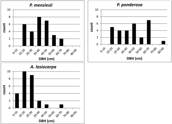
Fig. 2. DBH size class distribution of sample trees by species.
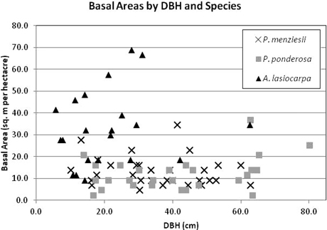
Fig. 3. Stand basal area (BA) by DBH and species of sample trees. BA was calculated using a 10 ft acre–1 factor angle gauge from the sample tree location, and included the sampled tree. Seven sample trees missing BA data not included.
Before scanning, vegetation obstructing the line of sight between the laser and a target tree was removed using chainsaws and/or hand tools – from grasses and shrubs at the base of the bole, to neighboring trees that impinged (visually or physically) upon the sample tree’s crown. From the perspective of the laser, the base of bole to top of crown and the entire width of the crown were isolated from other vegetation.
In total, 30 P. menziesii, 29 P. ponderosa, and 27 A. lasiocarpa were scanned. Trees were scanned using an Optech ILRIS 36D HD discrete return, time-of-flight terrestrial laser scanner. The laser was mounted on a pan-tilt base atop a level tripod (Fig. 4). The laser emits energy at 1535 nm wavelength with a 0.008594° beam divergence, resulting in a beam diameter of 29 mm at 100 m (16 mm at 25 m). Sampling was executed at 10 000Hz in a serpentine pattern from bottom to top. The laser records position and intensity (x, y, z, i) for each return; for this study, only first returns were recorded and analyzed. The desired spot-spacing (the distance between the center point of adjacent pulses) for all scans was 4 mm; actual values ranged from 3.6–5.6 mm, with a median value of 3.9 mm. This value represented maximum data richness for per–tree scan times of < 1 hour. The scanner was positioned at distances ranging from 8.2–54.9 m from the target with a median distance of 23.28 m. Although constant range would have been optimal, viewshed constraints (e.g. topography or nonremovable adjacent trees) resulted in 54% of the scans completed at ranges of 15–30 m, 16% at ranges < 15 m and 30% at ranges > 30 m. Individual scan times ranged from just a few minutes to over 40 minutes depending on tree size and the number of scans needed to capture it. There were eight trees where viewshed constraints combined with the maximum tilt angle of the pan-tilt base to precluded capturing the entire tree in one scan. In these cases, multiple scans were needed to capture the bottom and top of a tree, and an area of overlap was included to allow subsequent merging of the scans.
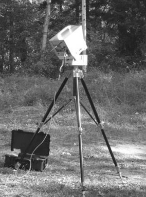
Fig. 4. The laser scan head is mounted on a pan-tilt base permitting bi-directional rotation. It is powered by a battery pack and scanning is controlled remotely through a hand-held device. Data is written to a USB-port on the rear panel of the scan head.
2.3 Data processing
Raw first returns were parsed into text files using Optech software. When multiple scans were needed to capture an entire tree, the upper scan was aligned to the lower scan using the Automated Best-fit Alignment and Comparison tool in Innovmetric’s Polyworks V11.0.1 IMAlign. The resultant rotation matrix was applied to the upper .xyz file using code executed in Excelis IDL 8.2.0 (Excelis Visual Information System 2007). The (unaltered) lower and (coordinate-shifted) upper scans were merged in a process that eliminated overlap between the scans. A user-defined plane that passed through the area of overlap was used to eliminate points above the plane (for lower scans) or below the plane (for upper scans). After removal of overlapping points, the scans were merged into one. Single scans that captured the entire tree in one scan did not require alignment or merging (Fig. 5).
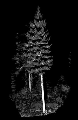
Fig. 5. An original single (unmerged) tree scan as initially visualized. Note that the sample tree in the foreground will be isolated by removing returns from other vegetation in the scene.
The tree of interest was isolated from each point cloud using a semi-automated process in IDL. The base of the target tree was visually identified in XYZ space and the remainder of the bole was delineated automatically from base to tip, with optional user correction to the proposed bole centroid (i.e., pith). Based on proximity to the finalized bole, a line of demarcation in XZ and YZ spaces (i.e., front view and side view) was created to separate points associated with the tree of interest from the surrounding point cloud. Again, user correction to a suggested delineation was allowed. In the YZ (side) view, laser returns behind the bole (away from the scanner) were excluded from the remainder of the point cloud. After isolation, the point cloud consisted of just the points from the half of the tree of interest that was closest to the scanner (Fig. 6).
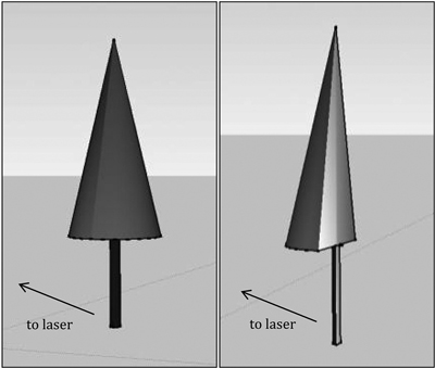
Fig. 6. Hypothetical extent of the original point cloud (left) and hemisphere of the tree closest to the scanner, after isolation.
2.4 Width percentile generation
Crown profiles were generated from 2D simplifications of the 3D point cloud. The Z coordinate of each return in the preprocessed point cloud was retained, while the X and Y coordinates of each return were combined into one value that described the horizontal Euclidean distance between that return and the bole centroid. This essentially “folded” the point cloud through a vertical rotation using the center of the bole as the axis, resulting in a 2D point distribution. In the new XY space, the center of the bole was the origin: the x-axis measured horizontal distance from the bole and the y-axis measured height above ground. A consequence of this transformation was the virtual straightening of bole sweep and lean.
In 0.25 m height increments, the distribution of returns in X space was used to calculate cumulative width percentiles for each height bin. Vertically following the points delineating a given percentile (e.g., the 50th, 95th, etc…) through each height increment yielded a crown profile for that percentile. Width percentiles were generated using code executed in IDL; all other crown profile analysis was complete in R (R Development Core Team 2013).
2.5 Crown delineation and rescaling
Characterization of crown shape and volume is predicated on identifying a crown base, which defines the “crown” to be modeled. Traditional measures such as CBH or HLC depend on a visual assessment of the tree that is subject to the assessor’s skill and accuracy. Scan data provide the opportunity to derive an objective, repeatable measure of crown base, independent of field measures. The LiDAR crown base height (LBH) was defined as the lowest height at which one-half the maximum value of the 95th crown width percentile was reached. Thus, if the maximum width of the 95th percentile was 4.2 m (i.e. the widest part of the crown), then the height where the 95th width percentile was 2.1 m was used as the crown base. This metric was chosen for its balance of simplicity and correlation with field measures of CBH and HLC from a large, but not exhaustive pool of model variants.
The LBH was used to separate the points as crown and below-crown, and the lower subset (the branchless bole) was discarded. For every tree, the retained (crown) 95th width percentile points were vertically rescaled between 0–1 to facilitate comparisons among trees of different crown lengths. First, the minimum height attributed to “crown” points (the minimum z) was subtracted from all the height values, and those results were divided by the total crown length (the maximum crown z minus the minimum crown z). Longer crowns had a greater number of width percentile observations than shorter crowns due to different numbers of 0.25 m height bins within the original crowns. The width values were rescaled proportionate to the original crown length for each tree by dividing each x coordinate (representing the crown width as the distance from the bole) by the crown length as calculated above. Thus, the crown percentiles were both scalable (because width was related to height) and comparable among trees of different original crown lengths.
2.6 Crown profile modeling
After rescaling, the 95th width percentile points for all trees of a single species were aggregated into one composite representation of the 95th width percentile. Past studies have used a variety of mathematical models to predict crown width, including parabolic forms (Biging and Wensel 1990) and polynomials (Baldwin and Peterson 1997; Hann 1999), with little consensus and few ties to other canopy parameter models. Conversely, beta and Weibull curves have been used to model foliage distribution at the tree and branch level (Mori and Hagihara 1991; Kershaw and Maguire 1996; and Maguire and Bennett 1996; Saito et al. 2004), a characteristic that can reasonably be expected to be tied to the ultimate extent of the foliage (i.e. the outer crown profile). The beta and Weibull functions, respectively, are given by


where x = crown width and z = vertical distance from crown base (height within the crown).
The beta parameters are defined as:
a and b = distribution shape parameters
ß = the beta function, a normalization constant
The Weibull parameters are defined as:
a = distribution scale parameter
b = distribution shape parameter
e = mathematical constant approximately equal to 2.71828
In this study, modified beta and Weibull curves were fit to the aggregated points to model crown profiles for each species. An additional scaling term (“c”) was added to both equations to fit the curves to the x-values of the points when the z-values (crown lengths) were constrained 0–1. This was necessary because for crown modeling purposes these functions need not be constrained to integrate to 1 as they must for probability modeling. The addition of this scaling factor resulted in a 3-parameter beta

and a 3-parameter Weibull function

where the variables are as defined above.
Inasmuch as the choice of the 95th width percentile to define the crown envelope was arbitrary, aggregate crown profile curves were also fit to the 91st and 99th width percentile point sets and compared. Lastly, simple geometric solids typically used by vegetation modelers (cones and cylinders) were also used to represent tree profiles. Various approaches have been used to fit these simple geometries to tree crowns. Canham et al. (1999) used cylinders whose radii were the average of the two longest perpendicular radii of the outermost crown projection to model nine species (both coniferous and deciduous). Mell et al. (2009) used cones whose diameters were based on the furthest extent of branch tips at the bottom of the crown (not necessarily the absolute lowest branches) to model tree-farm grown P. menziesii. Mawson et al. (1976) used cones based on the radius at the bottom of the crown, but noted that along the vertical extent of the crown, the widths of the actual trees exceeded the extent of the modeled profile. In this study, cones were shaped so that the radius of the cone at half the max height (0.5 after rescaling) was the median value of the aggregate 95th width percentile points between heights of 0.45 and 0.55 to address the shortcomings identified in previous studies. The radius of the cylinders was set using the same criteria. Those radii were: P. menziesii –0.160, P. ponderosa –0.178, A. lasiocarpa –0.782 (expressed as proportion of crown length; here crown length is 1).
2.7 Goodness of fit analysis
Leave-one-tree-out cross validation was used within each species to assess curve fit using mean absolute error (MAE). Specifically, after each tree’s 95th percentile width points were iteratively removed from the aggregated 95th width percentile point set, beta and Weibull curves were fit to the remaining width percentile points and the predicted widths at the reserved tree points were calculated using those fitted curves. MAE was calculated by subtracting the predicted width value for each reserved 95th width percentile point from the actual width value, and taking the absolute value of the result. These absolute errors for all width percentiles were then averaged over all each species set (not on a per-tree basis) to determine MAE. A minimum of 1400 absolute errors were averaged for each species.
The MAE metric was used for two reasons. First, using the absolute error allows a simple interpretation of the error statistic, in the same dimension as the data. The error metric is the potential crown width error; because crown width is rescaled relative to crown length (i.e., proportionate to crown length), the error can also be interpreted as a function of crown length. Second, MAE is less sensitive to outliers than the root mean squared error (RMSE) that is also dimensioned relative to the original data.
Lastly, the fit of each species’ final modeled curve (generated using all the data) was assessed against the aggregated 95th width percentile points for that species, as well as every other species and their simplified geometric (conic and cylindrical) forms. In all cases, the MAE statistic was used as the goodness-of-fit metric. Two-tailed Student’s t-tests were used to evaluate the differences in MAEs between modeled profiles, testing the curves’ species-specificity.
3 Results
3.1 Crown base delineation
The first objective of this study was to determine an objective, repeatable measure of crown base using TLS and assess any differences among TLS-derived and field-measured crown base metrics. For P. ponderosa and P. menziesii, both field-measured and TLS-derived crown base values had a fairly even distribution between the minimum and maximum values for each species (0.9–14.1 and 1.0–21.9 m, respectively). The distribution of crown base values (both field-measured and TLS-derived) in A. lasiocarpa was skewed toward the low end of the range of base heights, and 80% of these trees had a CBH less than 3.8 m. In all species, LBH estimated from TLS data was consistently lower than CBH measured in situ with the TruPulse rangefinder. In trees with low crown bases, LBH was smaller than field-measured HLC; in trees with high crown bases, LBH was higher than HLC. This trend was weaker in P. ponderosa than the other two species.
P. menziesii and A. lasiocarpa showed moderate correlations between TSL-derived LBH and both of the field-measured crown base metrics (R = 0.65–0.72); the correlation in P. ponderosa was strong (R = 0.97). The disparity between field-measured and TLS-derived crown base metrics was largely due to the presence of dead branches below the live crown; these tend to reduce LBH, but do not impact field assessments of CBH and HLC. This was most common in P. menziesii, and was also seen in some trees of A. lasiocarpa, but did not occur in P. ponderosa where dead branches are less common.
3.2 Crown profiles
After determining the LBH for each tree, the points comprising the 95th width percentiles of each tree’s crown were aggregated by species (Fig. 7). Modified beta and Weibull curves were fit to the aggregate percentile width points (at each height bin) for each species. The parameters for the curves generated from the aggregate 95th percentile width points are given in Table 2. Credibility for use of aggregated data is derived from the visual and statistical characteristics of equation parameters as a function of crown length for individual trees (Fig. 8 and Table 3).
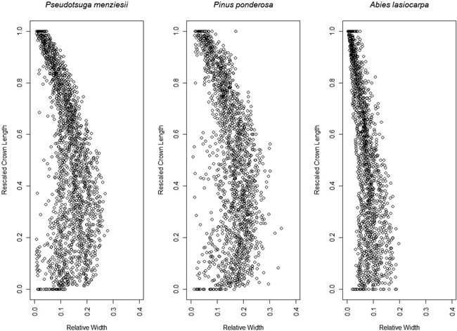
Fig. 7. Aggregate 95th width percentile points for each species, after rescaling crown length 0–1 and the crown width relative to the crown length.
| Table 2. Equation parameters for the aggregate 95th percentile points of each species. | ||
| Species | Beta | Weibull |
| P. menziesii | a = 1.2405 b = 1.5580 c = 0.1286 | a = 1.4043 b = 0.6610 c = 0.1540 |
| P. ponderosa | a = 1.1821 b = 1.4627 c = 0.1528 | a = 1.3266 b = 0.7241 c = 0.1943 |
| A. lasiocarpa | a = 1.1250 b = 1.6973 c = 0.0718 | a = 1.2677 b = 0.5780 c = 0.0832 |
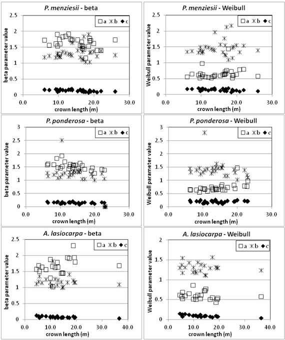
Fig. 8. Parameters for Weibull and beta curves of individual trees related to crown length. Note variations in axes among plots.
| Table 3. Each equation parameter (a, b, c for both beta and Weibull curves) was plotted against the structure and environmental variables of crown length, DBH and basal area. The table below reports the slope of the fitted linear regression and, in parentheses, two standard errors of the slope. | ||||||
| Beta parameters | Weibull parameters | |||||
| a | b | c | a | b | c | |
| P. menziesii | ||||||
| Crown length | –0.009 (0.014) | 0.007 (0.016) | –0.004 (0.002) | 0.007 (0.014) | 0.008 (0.020) | –0.004 (0.002) |
| DBH | 0.000 (0.004) | 0.002 (0.005) | 0.000 (0.001) | 0.000 (0.005) | 0.002 (0.007) | –0.001 (0.001) |
| Basal area | 0.002 (0.010) | –0.002 (0.011) | 0.001 (0.002) | –0.000 (0.010) | –0.004 (0.014) | 0.001 (0.002) |
| A. lasiocarpa | ||||||
| Crown length | 0.012 (0.017) | –0.003 (0.011) | –0.002 (0.001) | –0.003 (0.007) | –0.004 (0.008) | –0.003 (0.001) |
| DBH | 0.005 (0.008) | –0.001 (0.006) | –0.001 (0.001) | –0.001 (0.003) | –0.002 (0.004) | –0.001 (0.001) |
| Basal area | –0.004 (0.007) | –0.002 (0.005) | –0.001 (0.001) | 0.003 (0.002) | 0.000 (0.003) | 0.000 (0.001) |
| P. ponderosa | ||||||
| Crown length | –0.019 (0.011) | –0.013 (0.024) | –0.002 (0.003) | 0.018 (0.013) | –0.017 (0.027) | 0.001 (0.004) |
| DBH | –0.004 (0.003) | –0.002 (0.006) | 0.000 (0.001) | 0.002 (0.003) | –0.003 (0.006) | 0.000 (0.001) |
| Basal area | –0.019 (0.013) | –0.011 (0.028) | 0.001 (0.003) | 0.013 (0.016) | –0.014 (0.031) | 0.003 (0.004) |
The 95th percentile width did not produce beta or Weibull profiles that were appreciably different from those fitted to the 91st or 99th percentiles (Figs. 9 and 10). The resultant volumes derived from rotation of each profile relative to the volume produced using the 95th width percentile are consistent across species, with a slightly greater difference in volume between the 95th and 99th percentile curves than between the 91st and 95th (Fig. 11). In all but one case, the volumetric impacts due to percentile choice were minor compared to the volumetric differences between beta or Weibull profiles and conic or cylindrical forms. The exception to this pattern was the crown volume of A. lasiocarpa when modeled as a cylinder; volumetrically, this model fell between the values from the 95th and 99th percentile curves. As crowns are scaled up from a unit length, the relative crown volumes remain consistent, although the absolute differences among volumes from different models increase.
The beta curves (Fig. 9) have a flatter “belly” and a steeper base than the Weibull curves, a convex shape to the lower and upper portions of the curve, and a return to zero at the top of the crown profile. The Weibull curves (Fig. 10) have a rounder “belly”, convex lower portions and slightly concave upper portions, and tops that do not return to an x-axis value of zero (an inherent property of the unbounded Weibull distribution). In all species, the uppermost portion of the Weibull curve overestimates the crown width because the curve does not return to zero at the tree tip.
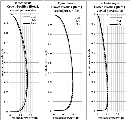
Fig. 9. Beta (modified) curves modeled on the 91st, 95th or 99th width percentile points for each species. Because the axes have been rescaled, they are considered unitless.
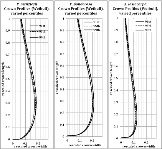
Fig. 10. Weibull (modified) curves modeled on the 91st, 95th or 99th width percentile points for each species. Because the axes have been rescaled, they are considered unitless.
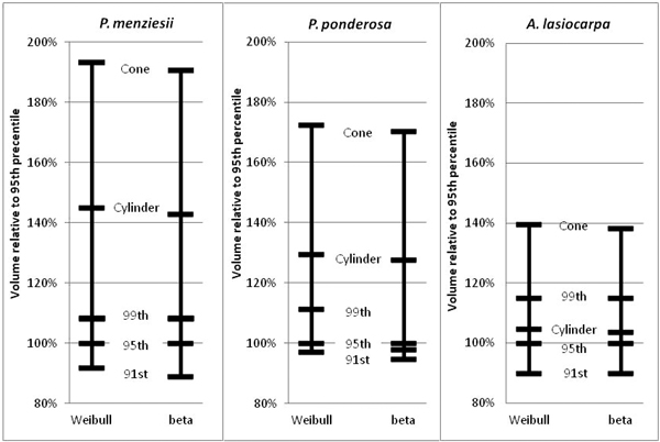
Fig. 11. Relative volume comparisons. For each species, beta and Weibull curves modeled on the 95th width percentiles were used to calculate “base” volumes. Then, volumes calculated from the 91st and 99th width percentile profile curves, and the modeled cones and cylinders for each species were compared to the base cases.
3.3 Goodness of fit analysis
The mean absolute error (MAE) from differencing each species’ 95th width percentile points from their respective modeled curve predictions is reported in Tables 4 and 5. The MAEs reported for each species when the modeled profile for the same species is applied come from cross-validation. In every case, the width percentile points of a species are best predicted by the curve calibrated for that species and the loss of accuracy that results from applying one species’ fitted profile to another are statistically significant (Fig. 12). It is not known if a curve from one species better fits an individual sample tree of another species because all data for a species were aggregated.
| Table 4. Mean absolute error (MAE) for predictions made by the beta curve of a species for the 95th width percentile points of each tree. P-values were calculated in R. | |||||
| Beta MAE | Modeled curve predictor species/shape | ||||
| Reference species 95th width percentile points | P. menziesii | P. ponderosa | A. lasiocarpa | Cone | Cylinder |
| P. menziesii | 0.034 p = na | 0.039 p<0.001 | 0.062 p<0.001 | 0.066 p<0.001 | 0.054 p<0.001 |
| P. ponderosa | 0.041 p<0.001 | 0.035 p = na | 0.084 p<0.001 | 0.075 p<0.001 | 0.052 p<0.001 |
| A. lasiocarpa | 0.059 p<0.001 | 0.082 p<0.001 | 0.022 p = na | 0.027 p<0.001 | 0.031 p<0.001 |
| Table 5. Mean absolute error (MAE) for predictions made by the Weibull curve of a species for the 95th width percentile points of each tree. P-values were calculated in R. | |||||
| Weibull MAE | Modeled curve predictor species/shape | ||||
| Reference species 95th width percentile points | P. menziesii | P. ponderosa | A. lasiocarpa | Cone | Cylinder |
| P. menziesii | 0.036 p = na | 0.040 p<0.001 | 0.062 p<0.001 | 0.066 p<0.001 | 0.054 p<0.001 |
| P. ponderosa | 0.043 p<0.001 | 0.037 p = na | 0.083 p<0.001 | 0.075 p<0.001 | 0.052 p<0.001 |
| A. lasiocarpa | 0.059 p<0.001 | 0.082 p<0.001 | 0.023 p = na | 0.027 p<0.001 | 0.031 p<0.001 |
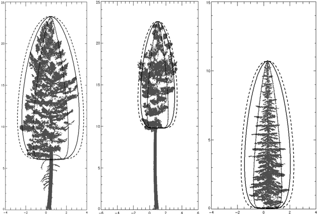
Fig. 12. Three species beta curves on one tree of each species (height and width expressed in meters). L to R – P. menziesii, P. ponderosa, A. lasiocarpa. P. menziesii curve is solid line, P. ponderosa curve is dashed line and A. lasiocarpa curve is dotted line. Each curve was generated using species’ parameters with crown length for the individual trees pictured.
Comparisons of aggregate 95th width percentile points with simple geometric shapes showed that a cylinder produced less error in P. menziesii than the A. lasiocarpa beta or Weibull curve. Both a cone and cylinder produced less error in P. ponderosa than did the A. lasiocarpa curves. The cone and cylinder produced less error for A. lasiocarpa 95th width percentile points than did the P. menziesii or P. ponderosa beta or Weibull curves. Although all of the curves were distinct, those of P. menziesii and P. ponderosa were more similar to each other and to some simple geometries than they were to A. lasiocarpa. The beta curves of P. menziesii and P. ponderosa produced less error than the Weibull curves; there was no difference in accuracy between beta and Weibull curves for A. lasiocarpa.
4 Discussion
The primary goal of this work was to identify species-specific models of crown shape and volume. Our approach allows prediction of a tree’s crown shape from crown length alone – an easily measured or estimated metric. Other TLS research (e.g., Fernandez-Sarria et al. 2013) has employed voxels, convex hulls and slices to produce volume estimates for individual trees, but these measures still require some method of generalization (e.g. curve fitting) to obtain predictive functions. A first step in the latter case may be to statistically relate estimated volume to an easily measured dimension such as DBH or crown length. This approach may allow prediction of total crown volume but not crown shape. The modeled shapes in our study (beta, Weibull and simple geometries) were assessed in terms of the error (as quantified by MAE) produced by each curve. The best-fit of the beta curve was largely driven by its flexibility in describing the curvature of profiles (as compared with simple geometric solids) and its convergence to zero crown width in the upper third of the modeled profile (as compared with the Weibull).
The curves presented were estimated from a sample of trees that spanned a range of conditions and sizes. As noted previously, however, not every site/size combination was accounted for. Other studies of tree crown shape have noted differences in crown form associated with woody-frame structure in Fraxinus pennsylvanica (Remphrey et al. 1987) and crown position in Pinus taeda (Zeide and Gresham 1991). However, Marshall et al. (2003) detected no relationship between social position and crown shape in Tsuga heterophylla. In our study, we intentionally limited variation in bole structure (no forking, etc.) which would thus constrain shape variation due to frame structure. The variety of tree sizes, crown lengths, and basal areas in our study spans a range of growing environments from competitive to open, although it is unlikely that every environment is represented equally. The absence of relationships between model parameters and crown length (Fig. 8), DBH, and basal area (Table 3) indicate that crown shape is not strongly conditioned by size and site factors, which supports the general applicability of the findings but also may reflect sample bias toward more open stand conditions and exposed tree crowns. The crown profile models derived nonetheless represent the best available information for the three species examined with the caveat that trees growing in competitive environments may be underrepresented in the samples used to derive their crown shapes. A more detailed assessment of the impact of environmental variables on crown shape such as tree density, site productivity, and terrain is not supported by the sample of trees or the field data collection protocols but would be of interest in future work.
Although our study did not explicitly characterize neighborhood structures around sample trees beyond basal area, recent literature points to tree neighborhood characteristics as fundamental to crown size and shape of individual trees. For example, competition for light tends produces asymmetric canopies in heterogeneous structures with direction of canopy plasticity predictable from height and distance of neighbor trees (Seidel et al. 2011). Bayer et al. (2013) used TLS to skeletonize branch structure of trees and showed that crown volume of Norway spruce was larger in stands mixed with beech than in pure stands due to longer branch lengths, while beech in the same environments exhibited differing branch numbers, lengths, and angles. It is clear from these works that the feedbacks between tree growth, forest structure, and environment are very complex and at least some of the variability in crown shapes observed in our study are due to both intra- and interspecific competition integrated over the time of stand development.
Folding the original 3D data based on distance to bole center is a computationally efficient way to integrate a hemisphere of data. Because of this integration, the resultant 100th percentile is not necessarily a maximum extent that would be created from any single vertical crown slice. Using a position interior to the 100th percentile compensates somewhat for horizontally asymmetrical crowns where branches on one side are notably longer than those on another portion of the crown. For example, the 95th percentile of an asymmetrical crown will be shrunk toward the bole, as compared to the same percentile of a symmetrical long-branched crown. Additionally, the folding technique used to translate the 3D point cloud into 2D rotates branches into within-canopy gaps that contribute to canopy complexity. The effect of this “filling in” on the modeled external profile is not well-defined. In short, the exact relationship between a profile produced from folded point sets and one produced by averaging a series of individual profiles from the 3D crown is unknown, but we speculate it to be similar based on comparison of predicted crown profiles and the native point clouds (Fig. 13). Lastly, it is worth considering that the half-tree scans utilized in this study do not characterize full crown asymmetry and models derived from them may show less variability than those from full tree scans.
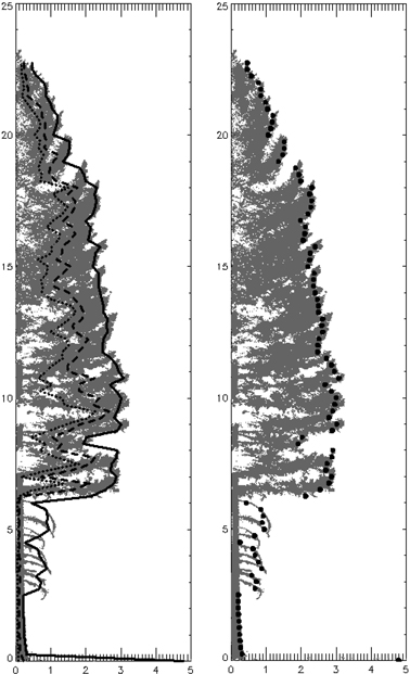
Fig. 13. Folded P. menziesii with 25th (dotted), 50th (dashed) and 95th (solid) width percentiles. Right image shows 95th percentile displayed as points (at the 0.25 m height increment bins).
Better reconciliation of TLS-derived and field-measured crown base height than is produced in this study is constrained by the inability of the laser to easily distinguish live from dead branches. A metric derived solely from TLS data is desirable because it provides consistency for a measurement that can be difficult to make in the field. The LBH used here was based on the presence/absence of crown material, and tended to be lower than the field definitions, which are based solely on live material. The best correlation among the measures was found in P. ponderosa, which self-prunes readily and does not typically carry a large dead branch load. It was important to establish a consistent measure of crown base because that defines the crown length and, in turn, the scaling factor for the crown profile curves. However, other better-performing crown base metrics may be identified in the future, perhaps using laser intensity data to identify live crown. Seielstad et al. (2011) and Béland et al. (2011) have each shown that laser intensity data can be used to distinguish foliage from branch wood in both conifer and broadleaf specimens using similar instruments and techniques.
From a modeling perspective, it is beneficial to have the ability to predict biomass from an easily obtainable measure such as DBH, predict crown shape from a single metric such as crown length, and to be able to realistically distribute predicted biomass within a predicted crown envelope. Our work addresses the middle step, and follow-on work will examine the internal arrangement of material in terms of a gradient from bole to crown hull and the internal clumpiness of biomass. One potential challenge in future work is the issue of occlusion – the depth of penetration the laser is able to achieve into dense crowns. In our work, the similarities between the 91st, 95th and 99th percentiles suggest that most of the laser returns are from the outer edges of the tree and support the argument that our profiles characterize the outer shell of the crown. However, when attempting to characterize the internal arrangement of material, one must consider the potential for occlusion and determine whether there are few laser returns from the inner crown because there is little material there, or because there are few laser pulses that reach those areas.
Occlusion remains one of the most confounding aspects of TLS of forests. It has been addressed in varying degrees by scanning objects many times from different perspectives (e.g., Hosoi and Omasa, 2006) and by modeling occluded space with data from light transmission models (e.g., Béland et al. 2011). The former approach has serious limitations in field settings due to inevitable viewshed constraints and long set-up and scan times. Further, multiple scans of natural features such as trees are both difficult to align and produce datasets with variable beam-target geometry across the scene. In our study, these factors were largely overcome by scanning trees from a single perspective and holding scanning parameters near constant, but at the cost of undersampling trees growing in competitive environments, ignoring half the crown of each tree scanned, and assuming that most reflections come from the outer hull of the tree. Although modeling methods are becoming increasingly adept at identifying occlusion (e.g., Côté et al. 2009), filling shadowed volumes with meaningful biophysical estimates is a work in progress (Béland et al. 2011). Characterizing internal features of tree crowns would benefit from using lasers with very small beam diameters that remain relatively invariant with range. The Optech ILRIS instrument used in this study does not meet these requirements as well as some other scanners used in forestry applications. In sum, the problem of occlusion will require considerable additional investigation by the TLS research community.
Overall, using TLS can facilitate capturing large and detailed data sets and overcomes many of the issues associated with photographic interpretation, with a few noteworthy drawbacks. The time commitment for field work and data processing, the training required for operation of the equipment and software, and the financial outlay associated with the technology are considerable. Although each tree of interest was not destructively sampled, basic clearing of the line-of-sight and adjacent vegetation was time consuming (up to two hours per tree in very dense stands or those with heavy underbrush). Once clear, laser scanning is more time intensive than photography (up to 40 minutes for large trees). Additionally, the laser operation and data processing required detailed training that is more complex than traditional field methods, and utilized equipment that is more costly than manual tools and photographic gear. Thus the current trade-offs for detailed crown capture in three dimensions are time expenditures (training, site preparation, data capture and processing) and monetary costs for instrumentation. TLS may best be used to develop individual tree models for incorporation into other models or studies, rather than as a common field-sampling tool. Studies like this one can be used to exploit the capabilities of laser scanning, inform more complex models and simulations, and preclude the need to collect field data on crown structure for every project.
5 Conclusions
As noted previously, crown profiles have been modeled using several methods, each with their own limitations. TLS is able to capture the crown extent in three dimensions, without destructive sampling, overcoming many of those limitations. By folding 3-dimensional data into two dimensions, information about the extent of the entire crown (not just one slice) is retained. For the three species sampled here (P. menziesii, P. ponderosa, and A. lasiocarpa), crown profiles were found to be species-specific, and best modeled using either a modified beta or Weibull curve tailored to that species. Importantly, the crown profile was modeled as a function of vertical position within the crown, and requires only crown length for implementation.
The ability of TLS to provide a detailed representation of the tree lends itself well to a direct calculation of crown profile. Roeh and Maguire (1997) chose to use indirect methods because of the “numerous logistical difficulties” associated with “direct measurement of crown diameters at different heights.” This challenge is well addressed by the use of TLS. Previous studies employing direct measurements relied on limited samples of crown width, measured in the field on felled trees (Doruska and Mays 1998 [7 sampled widths]; Hann 1999 [10 sampled widths]; Marshall et al. 2003 [10 sampled widths]). In this study, we obtained 18–146 measures per tree, dependent on crown length (in 0.25 m increments), from crowns measured without destructive sampling, and incorporating data from an entire hemisphere of the tree crown. TLS demonstrated potential to be more than a novel way to take traditional measurements, and instead lends itself to data collection and processing techniques that improve our ability to describe external crown architecture.
Specifically, this work found that:
- An objective, repeatable canopy base metric is derivable solely from TLS data. This metric is consistently lower than field-measures of canopy base height as measured by USFS guidelines (USDA Forest Service 2009), likely due to its consideration of all branches, live or dead.
- The 95th width percentile is an adequate descriptor of the “outer” limits of the crown, and little variation in profile shape was seen using alternate width percentiles. The volumetric changes associated with using different width percentiles were smaller than those from using simple shapes (i.e. cones or cylinders), with one exception.
- For two species (P. menziesii, P. ponderosa), a scaled beta curve gave the most accurate fit to the aggregated 95th width percentile points, as measured using MAE and cross-validation. For one species (A. lasiocarpa), there was no difference in accuracy between beta and Weibull curves. In all cases, beta and Weibull curves produced significantly smaller errors than did cones or cylinders.
- Curves are species-specific, and interchanging curves among different species produces significantly poorer fits to observed crown profiles.
Acknowledgements
This study was supported by a grant from the Joint Fire Sciences Program (10-1-02-13) with assistance from the University of Montana National Center for Landscape Fire Analysis and the Wildland Fire Science Partnership. Special thanks to Eric Rowell and Mike Fowler for programming and fieldwork.
References
Affleck D.L.R., Keyes C.R., Goodburn J.M. (2012). Conifer crown fuel modeling: current limits and potential for improvement. Western Journal of Applied Forestry 27: 165–169. http://dx.doi.org/10.5849/wjaf.11-039.
Baldwin V., Peterson K. (1997). Predicting the crown shape of loblolly pine trees. Canadian Journal of Forest Research 27: 102–107.
Bayer D., Seifert S., Pretzsch H. (2013). Structural crown properties of Norway spruce (Picea abies [L.] Karst.) and European beech (Fagus sylvatica [L.]) in mixed versus pure stands revealed by terrestrial laser scanning. Trees 27: 1035–1047. http://dx.doi.org/10.1007/s00468-013-0854-4.
Béland M., Widlowski J., Fournier R.A., Côté J., Verstraete M.M. (2011). Estimating leaf area distribution in savanna trees from terrestrial LiDAR measurements. Agricultural and Forest Meteorology 151: 1252–1266. http://dx.doi.org/10.1016/j.agrformet.2011.05.004.
Biging G., Wensel L. (1990). Estimation of crown form for 6 conifer species of northern California. Canadian Journal of Forest Research 20: 1137–1142. http://dx.doi.org/10.1139/x90-151.
Canham C., Coates K., Bartemucci P., Quaglia S. (1999). Measurement and modeling of spatially explicit variation in light transmission through interior cedar-hemlock forests of British Columbia. Canadian Journal of Forest Research 29: 1775–1783. http://dx.doi.org/10.1139/cjfr-29-11-1775.
Clark M.L., Roberts D.A., Ewel J.J., Clark D.B. (2011). Estimation of tropical rain forest aboveground biomass with small-footprint lidar and hyperspectral sensors. Remote Sensing of Environment 115: 2931–2942. http://dx.doi.org/10.1016/j.rse.2010.08.029.
Cluzeau C., Legoff N., Ottorini J. (1994). Development of primary branches and crown profile of Fraxinus excelsior. Canadian Journal of Forest Research 24: 2315–2323. http://dx.doi.org/10.1139/x94-299.
Cochran P.H., Geist J.M., Clemens D.L., Clausnitzer R.R., Powell D.C. (1994). Suggested stocking levels for forest stands in northeastern Oregon and southeastern Washington. U.S. Department of Agriculture, Forest Service, Pacific Northwest Research Station, Research Note PNW-RM-513. 21 p.
Côté, J-F., Widlowski J., Fournier R.A., Verstraete M.M. (2009). The structural and radiative consistency of three-dimensional tree reconstructions from terrestrial lidar. Remote Sensing of Environment 113: 1067–1081. http://dx.doi.org/10.1016/j.rse.(2009).01.017.
Côté J.-F., Fournier R., Egli R. (2011). An architectural model of trees for estimation of forest structural attributes using terrestrial LiDAR. Environmental Modelling and Software 26: 761–777. http://dx.doi.org/10.1016/j.envsoft.2010.12.008.
Crecente-Campo F., Marshall P., LeMay V., Dieguez-Aranda U. (2009). A crown profile model for Pinus radiata D. Don in northwestern Spain. Forest Ecology and Management 257: 2370–2379. http://dx.doi.org/10.1016/j.foreco.(2009).03.038.
Da Silva D., Boudon F., Godin C., Sinoquet H. (2008). Multiscale framework for modeling and analyzing light interception by trees. Multiscale Modeling and Simulation 7: 910–933. http://dx.doi.org/10.1137/08071394X.
Danson F.M., Hetherington D., Morsdorf F., Koetz B., Allgoewer B. (2007). Forest canopy gap fraction from terrestrial laser scanning. IEEE Geoscience and Remote Sensing Letters 4: 157–160. http://dx.doi.org/10.1109/LGRS.(2006).887064.
Dassot M., Colin A., Santenoise P., Fournier M., Constant T. (2012). Terrestrial laser scanning for measuring the solid wood volume, including branches, of adult standing trees in the forest environment. Computers and Electronics in Agriculture 89: 86–93. http://dx.doi.org/10.1016/j.compag.(2012).08.005.
Delagrange S., Rochon P. (2011). Reconstruction and analysis of a deciduous sapling using digital photographs or terrestrial-LiDAR technology. Annals of Botany 108: 991–1000. http://dx.doi.org/10.1093/aob/mcr064.
Deleuze C., Herve J., Colin F., Ribeyrolles L. (1996). Modelling crown shape of Picea abies: spacing effects. Canadian Journal of Forest Research 26: 1957–1966. http://dx.doi.org/10.1139/x26-221.
Doruska P., Mays J. (1998). Crown profile modeling of loblolly pine by nonparametric regression analysis. Forest Science 44: 445–453.
Duursma R.A., Mäkelä A. (2007). Summary models for light interception and light-use efficiency of non-homogeneous canopies. Tree Physiology 27: 859–870.
Edminster C.B. (1987). Growth and yield of subalpine conifer stands in the central Rocky Mountains. In: Troendle C.A., Kaufmann M.R., Hamre R.H., & Winokur R.P. (tech. coords.). Management of subalpine forests: building on 50 years of research. U.S. Department of Agriculture, Forest Service, Rocky Mountain Forest and Range Experiment Station, General Technical Report RM-GTR-149. p. 33–40.
Exelis Visual Information Solutions. (2007). Interactive data language (IDL): version 8.0. Boulder, CO.
Fernández-Sarría A., Velázquez-Martí B., Sajdak M., Martínez L., Estornell J. (2013). Residual biomass calculation from individual tree architecture using terrestrial laser scanner and ground-level measurements. Computers and Electronics in Agriculture 93: 90–97. http://dx.doi.org/10.1016/j.compag.(2013).01.012.
Gill S., Biging G. (2002). Autoregressive moving average models of conifer crown profiles. Journal of Agricultural Biological and Environmental Statistics 7: 558–573. http://dx.doi.org/10.1198/108571102762.
Hann D. (1999). An adjustable predictor of crown profile for stand-grown Douglas-fir trees. Forest Science 45: 217–225.
Henning J.G., Radtke P.J. (2006). Ground-based laser imaging for assessing three-dimensional forest canopy structure. Photogrammetric Engineering and Remote Sensing 72: 1349–1358.
Hiers J.K., O’Brien J.J., Mitchell R.J., Grego J.M., Loudermilk E.L. (2009). The wildland fuel cell concept: an approach to characterize fine-scale variation in fuels and fire in frequently burned longleaf pine forests. International Journal of Wildland Fire18: 315–325. http://dx.doi.org/10.1071/WF08084.
Hoffman C., Morgan P., Mell W., Parsons R., Strand E.K., Cook S. (2012). Numerical simulation of crown fire hazard immediately after bark beetle-caused mortality in lodgepole pine forests. Forest Science 58: 178–188. http://dx.doi.org/10.5849/forsci.10-137.
Hosoi F., Omasa K. (2006). Voxel-based 3-D modeling of individual trees for estimating leaf area density using high-resolution portable scanning lidar. IEEE Transactions on Geoscience and Remote Sensing 44: 3610–3618. http://dx.doi.org/10.1109/TGRS.(2006).881743.
Kershaw J.A., Maguire D.A. (1996). Crown structure in western hemlock, Douglas fir and grand fir in western Washington: horizontal distribution of foliage within branches. Canadian Journal of Forest Research 26: 128–142. http://dx.doi.org/10.1139/x26-014.
Lesak A.A., Radeloff V.C., Hawbaker T.J., Pidgeon A.M., Gobakken T., Contrucci K. (2011). Modeling forest songbird species richness using LiDAR-derived measures of forest structure. Remote Sensing of Environment 115: 2823–2835. http://dx.doi.org/10.1016/j.rse.(2011).01.025.
Lovell J., Jupp D., Culvenor D., Coops N. (2003). Using airborne and ground-based ranging lidar to measure canopy structure in Australian forests RID B-1326-(2012). Canadian Journal of Remote Sensing 29: 607–622.
Maguire D.A., Bennett W.S. (1996). Patterns in vertical distribution of foliage in young coastal Douglas-fir. Canadian Journal of Forest Research 26: 1991-(2005). http://dx.doi.org/10.1139/x26-225.
Marshall D.D., Johnson G.P., Hann D.W. (2003). Crown profile equations for stand-grown western hemlock trees in northwestern Oregon. Canadian Journal of Forest Research 33: 2059–2066. http://dx.doi.org/10.1139/X03-126.
Mawson J.C., Thomas J.W., DeGraaf R.M. (1976). Program HTVOL: the determination of tree crown volume by layers. USDA Forest Service, Research Paper NE-RP-354.
Mell W., Maranghides A., McDermott R., Manzello S.L. (2009). Numerical simulation and experiments of burning douglas fir trees. Combustion and Flame 156: 2023–2041. http://dx.doi.org/10.1016/j.combustflame.(2009).06.015.
Moore J.A., Mike P.G., Vander Ploeg J.L. (1991). Nitrogen fertilizer response of Rocky Mountain Douglas-fir by geographic area across the Inland Northwest. Western Journal of Applied Forestry 6: 94–98.
Moorthy I., Miller J.R., Hu B., Chen J., Li Q. (2008). Retrieving crown leaf area index from an individual tree using ground-based lidar data. Canadian Journal of Remote Sensing 34: 320–332.
Mori S., Hagihara A. (1991). Crown profile of foliage area characterized with the Weibull distribution in a Hinoki (Chamaecyparis obtusa) stand. Trees – Structure and Function 5: 149–152.
Oker-blom P., Kellomaki S. (1983). Effect of grouping of foliage on the within-stand and within-crown light regime – comparison of random and grouping canopy models. Agricultural Meteorology 28: 143–155. http://dx.doi.org/10.1016/0002-1571(83)90004-3.
Ottmar R.D., Blake J.I., Crolly W.T. (2012). Using fine-scale fuel measurements to assess wildland fuels, potential fire behavior and hazard mitigation treatments in the southeastern USA. Forest Ecology and Management 273: 1–3. http://dx.doi.org/10.1016/j.foreco.(2011).11.003.
Palminteri S., Powell G.V.N., Asner G.P., Peres C.A. (2012). LiDAR measurements of canopy structure predict spatial distribution of a tropical mature forest primate. Remote Sensing of Environment 127: 98–105. http://dx.doi.org/.1016/j.rse.(2012).08.014.
Parsons R.A., Mell W.E., McCauley P. (2011). Linking 3D spatial models of fuels and fire: effects of spatial heterogeneity on fire behavior. Ecological Modelling 222: 679–691. http://dx.doi.org/10.1016/j.ecolmodel.(2010).10.023.
Parveaud C., Chopard J., Dauzat J., Courbaud B., Auclair D. (2008). Modelling foliage characteristics in 3D tree crowns: influence on light interception and leaf irradiance. Trees – Structure and Function 22: 87–104. http://dx.doi.org/10.1007/s00468-007-0172-9.
Parresol B.R. (1999). Assessing tree and stand biomass: a review with examples and critical comparisons. Forest Science 45(4): 573–593.
R Development Core Team (2013). R: a language and environment for statistical computing. R Foundation for Statistical Computing, Vienna, Austria. ISBN 3-900051-07-0. http://www.R-project.org/. [Cited 6 Sep 2011].
Reinhardt E.D., Ryan K.C. (1988). Eight-year tree growth following prescribed under-burning in a western Montana Douglas-fir/western larch stand. U.S. Department of Agriculture, Forest Service, Intermountain Research Station, Research Note INT-387. 6 p.
Reinhardt E., Scott J., Gray K., Keane R. (2006). Estimating canopy fuel characteristics in five conifer stands in the western United States using tree and stand measurements. Canadian Journal of Forest Research 36: 2803–2814.
Remphrey W.R., Davidson C.G., Blouw M.J. (1987). A classification and analysis of crown form in green ash (Fraxinus pennsylvanica). Canadian Journal of Botany 65: 2188–2195.
Roeh R.L., Maguire D.A. (1997). Crown profile models based on branch attributes in coastal Douglas-fir. Forest Ecology and Management 96: 77–100. http://dx.doi.org/10.1016/S0378-1127(97)00033-9.
Rosell J.R., Sanz R. (2012). A review of methods and applications of the geometric characterization of tree crops in agricultural activities. Computers and Electronics in Agriculture 81: 124–141. http://dx.doi.org/10.1016/j.compag.(2011).09.007.
Saito S., Sato T., Kominami Y., Nagamatsu D., Kuramoto S., Sakai T., Tabuchi R., Sakai A. (2004). Modeling the vertical foliage distribution of an individual Castanopsis cuspidata (Thunb.) Schottky, a dominant broad-leaved tree in Japanese warm-temperate forest. Trees – Structure and Function 18: 486–491. http://dx.doi.org/10.1007/s00468-004-0338-7.
Sanz-Cortiella R., Llorens-Calveras J., Escola A., Arno-Satorra J., Ribes-Dasi M., Masip-Vilalta J., Camp F., Gracia-Aguila F., Solanelles-Batlle F., Planas-DeMarti S., Palleja-Cabre T., Palacin-Roca J., Gregorio-Lopez E., Del-Moral-Martinez I., Rosell-Polo J.R. (2011). Innovative LIDAR 3D dynamic measurement system to estimate fruit-tree leaf area. Sensors 11: 5769–5791. http://dx.doi.org/10.3390/s110605769.
Seidel D., Fleck S., Leuschner C., Hammet T. (2011). Review of ground-based methods to measure the distribution of biomass in forest canopies. Annals of Forest Science 68(2): 225–244. http://dx.doi.org/10.1007/s13595-0040-z.
Seidel D., Leuschner C. Muller A., Krause B. (2011). Crown plasticity in mixed forests – quantifying asymmetry as a measure of competition using terrestrial laser scanning. Forest Ecology and Management 261(11): 2123–2132. http://dx.doi.org/10.1016/j.foreco.2011.03.008.
Seielstad C., Stonesifer C., Rowell E., Queen L. (2011). Deriving fuel mass by size class in Douglas-fir (Pseudotsuga menziesii) using terrestrial laser scanning. Remote Sensing 3: 1691–1709. http://dx.doi.org/10.3390/rs3081691.
Skowronski N.S., Clark K.L., Duveneck M., Hom J. (2011). Three-dimensional canopy fuel loading predicted using upward and downward sensing LiDAR systems. Remote Sensing of Environment 115: 703–714. http://dx.doi.org/10.1016/j.rse.(2010).10.012.
Stage A.R., Renner D.L., Chapman R.C. (1988). Selected yield tables for plantations and natural stands in inland northwest forests. U.S. Department of Agriculture, Forest Service, Intermountain Research Station, Research Paper INT-394. 63 p.
Takeda T., Oguma H., Sano T., Yone Y., Fujinuma Y. (2008). Estimating the plant area density of a Japanese larch (Larix kaempferi Sarg.) plantation using a ground-based laser scanner. Agricultural and Forest Meteorology 148: 428–438. http://dx.doi.org/10.1016/j.agrformet.(2007).10.004.
USDA Forest Service. (2009). Field instructions: stand examination. Timber management data handbook FSH 2409.21h R-1. USDA, Forest Service, Region 1, Missoula, MT.
Vanclay J.K. (1994). Modeling forest growth and yield: applications fot mixed tropical forests. CAB International, Wallingford, UK.
VanderSchaaf C.L. (2008). Estimating understory vegetation response to multi-nutrient fertilization in Douglas-fir and ponderosa pine stands. Journal of Forest Research 13: 43–51.
Zeide B., Gresham C. (1991). Fractal dimensions of tree crowns in 3 loblolly pine plantations of coastal South Carolina. Canadian Journal of Forest Research 21: 1208–1212. http://dx.doi.org/10.1139/x91-169.
Total of 62 references
