Santiago Pereira,
Antonio Prieto,
Rafael Calama,
Luis Diaz-Balteiro 
Optimal management in Pinus pinea L. stands combining silvicultural schedules for timber and cone production
Pereira S., Prieto A., Calama R., Diaz-Balteiro L. (2015). Optimal management in Pinus pinea L. stands combining silvicultural schedules for timber and cone production. Silva Fennica vol. 49 no. 3 article id 1226. https://doi.org/10.14214/sf.1226
Highlights
- Three management scenarios are proposed to integrate timber and pine nuts
- Different silvicultural regimes for each output are addressed jointly
- Goal programming is used in order to solve forest management models
- In the mixed scenario, the area allocated to pine nuts should be notably greater.
Abstract
This work aimed to tackle a timber harvest scheduling problem by simultaneously integrating into the analysis two forestry products derived from the same species: the timber and the pine nut. For this purpose, three management scenarios were proposed: two in which each of the productions is maximised separately, and a third mixed where, in each management unit, the product to which the silvicultural effort should be devoted is decided. After defining a set of objectives, and optimising the rotation length, a multi-criteria model based on goal programming was considered since no feasible solutions have been obtained when employing linear programming. The results in our case study show how the feasible solutions reached can be more attractive for the manager. Specifically, the area to be devoted to timber and cone/pine-nut production was computed in a scenario where the optimal silviculture (oriented towards timber or pine nuts) in each stand was selected, and it was concluded that the area allocated to pine nuts should be notably greater. This situation is the opposite of the current management.
Keywords
forest management;
goal programming;
non-timber forest product
- Pereira, Technical University of Madrid, ETS Ingenieros de Montes, Ciudad Universitaria s/n, 28040 Madrid, Spain E-mail spereirasaez@gmail.com
- Prieto, Technical University of Madrid, ETS Ingenieros de Montes, Ciudad Universitaria s/n, 28040 Madrid, Spain E-mail antonio.prieto@upm.es
- Calama, Dpto. Selvicultura y Gestión Forestal, INIA-CIFOR, Ctra. A Coruña km 7.5, 28040 Madrid, Spain E-mail rcalama@inia.es
-
Diaz-Balteiro,
Technical University of Madrid, ETS Ingenieros de Montes, Ciudad Universitaria s/n, 28040 Madrid, Spain
E-mail
luis.diaz.balteiro@upm.es
Received 21 July 2014 Accepted 22 May 2015 Published 15 June 2015
Views 141897
Available at https://doi.org/10.14214/sf.1226 | Download PDF

Supplementary Files
1 Introduction
The Mediterranean stone pine, Pinus pinea L. (Pinaceae), is one of the most characteristic tree species of the Mediterranean forests and woodlands because of its singular umbrella shape, its ability to grow over dry, sandy soils, and the ancient use of its large, nutlike, edible seeds for human consumption. It is widely distributed throughout the Mediterranean basin, where, as a dominant species, it covers more than 700 000 ha (Mutke et al. 2012), mainly in Spain (450 000 ha), Portugal (90 000 ha), Turkey (50 000 ha) and Italy (40 000 ha). Although the autochthonous character of the species in the north-western Mediterranean has been widely demonstrated by fossil, palynological and archaeological evidence (Rubiales et al. 2010, 2011), the current natural area is difficult to determine, since it has been widely expanded in the last centuries (Mutke et al. 2012).
Stone pine forests have been used since ancient times as a source of timber, edible pine nuts, fuelwood, barks and resins. Besides, stone pine forests provide important ecological, landscape and recreational services, and, due to their capacity for growing over continental and coastal dunes, they have been widely used as protectors against soil erosion. Stone pine forests in Spain have been managed under multifunctional principles since the end of the 19th century (Romero-Gilsanz 1886). Bark extraction, resin tapping and pruning for fuelwood are abandoned practices in stone pine forests, and timber prices for the species have recently dropped so that cone production and pine-nut extraction have become the most interesting and profitable outputs from these forests in Spain (Ovando et al. 2010). Today, cone harvesting from the trees, subsequent industrial pine nut extraction and market processes are economic activities supporting more than 5000 jobs only in the inland regions of Spain. Extensive research and development have been conducted on the biology, ecology and silviculture of the species and, in particular, its cone and nut yield (Montero et al. 2008).
Unlike the main part of the species of the genus Pinus, the fruiting process in Pinus pinea covers a three-year period. Trees start to produce significant cone crops when they are over 20 years old, and maintain their production up to 140 to 150 years of age. Tree-level cone production is positively related to tree size (diameter and crown width), soil water holding capacity, social status of the tree and site index, while higher stocking reduces cone production (Calama et al. 2008). In short, Pinus pinea is a typical masting habit species, showing huge interannual variability in fruit production mainly ruled by climate factors, especially rainfall events occurring at key moments (bud induction and differentiation, and cone maturation) during the whole process, and secondary control by resource depletion (Mutke et al. 2005). Despite large spatial and temporal variability in cone production, the rate between the final end weight of pine nuts and weight of cones collected remains almost constant (4%, Montero et al. 2008). Thus the maximisation of pine-nut production is attained by means of maximising cone production, and throughout the text we will refer to the optimisation of cone/pine-nut production.
In temperate and boreal forests, non-timber forest products (NTFPs) may also be of great importance (Hallikainen et al. 2010). However, in the literature there are few examples of strategic forest planning models which have integrated other tangible production derived from NTFPs with timber production. Following Gautam and Devoe (2006) and Miina et al. (2010), the NTFPs ought to be integrated into management planning, although few studies illustrate how timber production could be affected by silviculture of NTFPs (Guariguata et al. 2010). Furthermore, another option would be to spatially separate the two productions, as suggested by Klimas et al. (2012).
In recent years, research into non-timber products, like mushroom production, has been included in forest planning through the use of optimisation tools. Thus, in Aldea et al. (2012) and De-Miguel et al. (2014a), it was shown that mushroom production is essentially compatible with optimisation of timber resources, contributing to the sustained yield of the forest. However, in these studies, the silvicultural models have been oriented only towards timber production. Palahí et al. (2009) defined a simulation model of thinnings and regenerative cuttings in two inventory plots in order to optimise the management of timber and mushrooms using the Hooke and Jeeves algorithm. The objective function maximises the net present value of the two products. The same algorithm has been used in other studies. Thus, Miina et al. (2010) analysed how the integration of bilberry production modified the optimal management of three stands in Finland, while in De-Miguel et al. (2014b) pine honeydew honey was optimised with timber production. Another NTFP that has been analysed with optimising tools is cork production. Thus, in Borges et al. (1997) and Costa et al. (2010), a linear programming (LP) problem formulated in order to optimise cork harvest scheduling can be found. These authors have included only one silviculture, associated with cork production. In addition, in Hjortsø and Stræde (2001), LP and discrete multi-criteria decision-making techniques (MCDMs) have been addressed to integrate berry and mushroom production in a case study in Lithuania. Finally, MCDMs have been used to determine potential harvesting sites for three edible ferns in Japan in Matsuura et al. (2014).
Today, in Spain, those forests where Pinus pinea is the main species are managed in order to achieve complete natural regeneration, in addition to certain restrictions associated with the landscape and protection of wildlife. However, decision-makers hesitate between choosing timber production or cone production silviculture. These silvicultures are integrated in rigid forest management planning, where the ideal of a normal forest still remains. Usually, the same orientation (timber or cone/pine-nut production) is adopted for the whole forest or for large groups of stands. In short, decision making related to choosing the best silvicultural alternative in order to obtain natural regeneration is not an easy task for forest managers (Manso et al. 2014). As a result, sometimes current planning is not implemented, natural regeneration is not achieved, cone production can be uncollected, and the decision-maker does not know how to integrate the two outputs using traditional European forest management methods.
To the best of our knowledge, no timber harvest scheduling problem using different silvicultural regimes for each output (timber and NTFP) has ever been addressed jointly. Thus, in some papers previously cited, the silviculture regimes are mainly oriented towards jointly optimising timber and NTFP on a stand scale. The main objective of this study was to obtain the best alternatives for managing each Pinus pinea stand while simultaneously optimising silvicultural options oriented towards timber or towards cone/pine-nut production on a forest scale. Thus, we have aimed to identify the optimal silvicultural regime for each stand. Furthermore, the methodology described can assess the opportunity cost of not taking an optimal management alternative associated with the silviculture chosen in each stand.
2 Material
2.1 Case study
The forest analysed (“Pinar del Común y Pinar de Propios y Valdeoliva”) is publicly owned. It covers 1396.5 ha and is located in the north of the province of Toledo (central Spain) on sandy, poor, acidic soils. Its altitude ranges between 550 and 850 metres above sea level. Slopes of between 3% and 12% predominate and in some specific areas they range from 12 to 24%. Stone pine constitutes the most abundant species in the forest, but there are also oak tree stands (Quercus ilex subsp. Ballota (Desf.) Samp.) and, less frequently, junipers (Juniperus oxycedrus L.). These pine trees commonly form grazing land stands, are of a low density, with trees with a large diameter and of a great age (100 to 150 years, with some individuals around 200 years). In the study area, the average stand density for Pinus pinea is 117 trees/ha, and the volume per hectare reaches 50.3 m3/ha (Prieto et al. 2004). Also, among other reasons, it presents scant regeneration due to pressure from cattle.
Its management began in 2004, applying classical European management methods (which are not based upon optimisation approaches), seeking to obtain a normal forest, and with silviculture oriented to timber production in the whole of the forest. However, in masting years when the cone production is high, the cone crop (on the tree) has been sold. The forest plan has been developed without using any optimisation techniques. The current structure of the forest can be defined as uneven-aged with patches or small even-aged groups. This means that there is no intimate mixture of trees of different age classes, but a mixture of even-aged groups occupying different areas, from 0.1 ha up to over 5 ha. Thus, the forest was initially divided into 133 stands, where even-aged groups of 3–4 different age classes can be found. We have defined a patch as being the aggregation of the groups from the same stand sharing the same age class, so that at the end each stand is subdivided into a number of different even-aged patches (more than 350 in the whole of the forest). Forest inventory information available at patch level includes the distribution of the frequencies of observed diameters, grouped by 5 cm diameter classes, as well as patch age and dominant height. Thus, each patch is associated with a site index focusing on timber production, defined by the dominant height at 100 years of age according to Calama et al.’s (2003) site index model for the species.
2.2 Economic variables
Given that the profitability of each of the management alternatives for each management unit will be calculated, it is necessary to compute, starting from the silvicultural plans (see Section 3.2.), both the income and payments expected throughout the planning horizon (100 years). With regard to the income, beginning with the pine nut, a price of 0.07 €/kg of cone (stumpage price) was taken, corresponding to the latest sale recorded in the forest. As we are focusing on the forest owner/forest manager point of view, we use the stumpage price of cones instead of the final price of pine nuts traded in the industry after the extractive process. The prices considered for the timber arose both from consulting timber merchants in areas near the forest, as well as information associated with other stone pine timber use in public forests. Thus, these stumpage prices are 14 €/m3 for the final cuttings and 4 €/m3 for timber from commercial thinnings. With regard to the payments, together with the costs of the silvicultural operations introduced in Table 1, others, associated with fencing pastures after the cutting (1216 €/ha), and the removal of fences in the 20th year after cutting (112.6 €/ha) have been taken into account. Besides, a cost of 8.4 €/ha has been included due to other operations to be carried out in the forest. These are all shown in Table 2. Finally, a real discount rate of 2% was taken. This rate has been used for long rotation forest species in Spain (Diaz-Balteiro and Romero 1998).
| Table 1. Silvicultural actions proposed for the two products. | ||
| TIMBER SCENARIO | ||
| Age | Operation | Intensity |
| 10 years | pre-commercial thinning | 350 trees/ha, with a density of 500 trees/ha after this treatment |
| 20 years | pruning | mainly in the lowest branches |
| 40 years | commercial thinning | low thinning, with a density of 225 trees/ha after this treatment |
| Rotation age (80–150 years) | clearcuts | leaving 10 seed trees by ha |
| CONE/PINE NUT SCENARIO | ||
| Age | Operation | Intensity |
| 10 years | pre-commercial thinning | 350 trees/ha, with a density of 500 trees/ha after this treatment |
| 15 years | pruning | lowest branches up to 40–60% of the height |
| 45 years | commercial thinning | low thinning, with a final density of 100 trees/ha after this treatment |
| Rotation age (80–150 years) | clearcuts | leaving 10 seed trees by ha |
| Table 2. Costs associated with each scenario. | ||
| TIMBER SCENARIO | ||
| Year | Operation | Cost |
| following final cutting | fenced to restrict grazing | 1126.16€/ha |
| 10 years | pre-commercial thinning | 285 €/ha |
| 20 years | pruning and removal of fence | 552.62 €/ha |
| 40 years | commercial thinning | 598 €/ha |
| CONE/PINE NUT SCENARIO | ||
| Year | Operation | Cost |
| following final cutting | fenced to restrict grazing | 1126.16€/ha |
| 10 years | pre-commercial thinning | 285 €/ha |
| 15 years | pruning | 440 €/ha |
| 20 years | removal of fence | 112.62€/ha |
| 45 years | commercial thinning | 870 €/ha |
3 Methods
3.1 PINEA2 model and applicability to forest case study
The evolution of the different patches in the forest “Pinar del Común y Pinar de Propios y Valdeoliva” under each management schedule was simulated using the PINEA2 model and software. PINEA2 (Calama et al. 2007) is an independent integrated single tree distance model simulating the growth and yield (timber and cones) of a pure stand of Pinus pinea under different management scenarios. Input variables for applying PINEA2 in the present work were breast height diameter of all the trees within the patch, patch age and dominant height. PINEA2 includes five modules (Fig. 1).
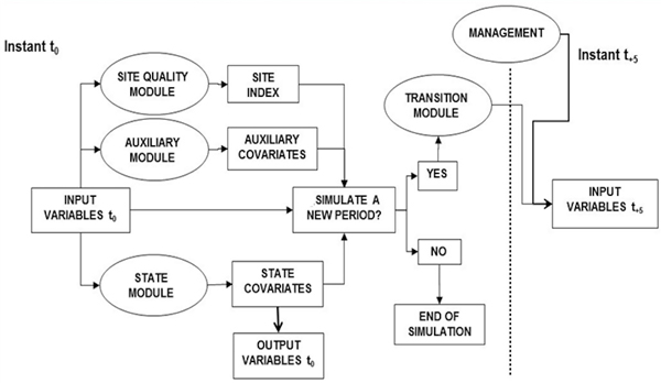
Fig. 1. Flow chart of PINEA2 model.
The state module includes different equations to predict tree size attributes, tree volume with end-size classification, tree biomass, and the average annual tree cone production (Calama et al. 2008). The transition module defines the future state of the patch, based on the current, by means of tree diameter and dominant height increment functions. Regarding natural regeneration, based on field observation and simulations carried out using the model by Manso et al. (2014), we assumed that complete regeneration was achieved within a 20-year period. In the case of mortality, current stocking is so low that it prevents self-thinning mortality (Montero and Candela 1998), thus only random mortality – assumed to occur at a rate of 1% every five years up to an age of 100 years, and at a rate of 3% over this age – has been considered. These percentages are based on the continuous monitoring of the net of permanent plots of Pinus pinea within the region used to construct the model. Finally, in the management module, PINEA2 allows one to propose different management schedules defined by thinning type, instant and intensity, and rotation length. As outputs of PINEA2, for each five-year simulation period, we obtained (i) stand attributes (ii) accumulated and standing volume, classified according to its end use, (iii) accumulated cone production per hectare, and (iv) accumulated and standing biomass defined by fractions and fixed CO2. The predicted weight of cones given by PINEA2 can be easily transformed into weight of pine nuts by applying a rate of 4% (Montero et al. 2008).
3.2 Proposed silvicultural schedules
Based on previous knowledge of silviculture and management for the species (e.g. Montero et al. 2008), two main silvicultural schedules are proposed, defined by their main production objective: timber or cones (and subsequently, pine nuts). Though Pinus pinea forests have been managed under multifunctionality and sustainability principles since ancient times, forest managers habitually must decide whether to orient their practices in order to promote one or another main production, since optimisation techniques are currently not applied in Spain. Thus, two simple management schedules have been proposed (see Table 1).
Initial stages are similar for both schedules. Patches under the regeneration phase are fenced to prevent grazing, and cone collection is prohibited to ensure enough seed source. Precommercial thinnings are oriented towards obtaining 500 stems/ha uniformly distributed throughout the area. The main differences are related to thinning and pruning operations. Cone-oriented management requires maintaining lower stocking from the earliest stages of stand development in order to promote and favour horizontal crown growth. Selective thinnings to favour the best 100 cone producers per hectare are thus applied, together with intensive stem pruning. On the other hand, timber production management is based on maintaining high standing stocks, so thinning from below up to 225 stems/ha is proposed and natural pruning favoured (Montero et al. 2008). From 20 years up to the regeneration cutting, the cones are cropped annually by using mechanical harvesters (vibrators). Natural regeneration is achieved by applying selective tree cutting by small patches, leaving 10 trees/ha to give initial protection to the seedlings. The rotation length can range between 80 and 150 years, and is the variable to be optimised on a stand scale. In order to avoid timber rot due to Phellinus pini, low rotation lengths are typical of timber-oriented stands, while cone production increases with age up to 140 to 150 years. Over this age, cone production is drastically reduced and mortality is increased.
3.3 Model I
The first step was to establish a strategic harvest scheduling model (Model I, following Johnson and Scheurman 1977). Three initial management scenarios were considered. Two of them implied the application of a silviculture oriented towards the same output (timber or cones/pine nuts), following the two main silvicultural schedules proposed, whereas in the third scenario the best silviculture choice (silviculture actions to promote either timber or cone/pine-nut production) in each stand was selected.
The set of prescriptions was defined according to the management unit chosen. Each stand was assigned an initial age, taken from the current forest management plan. The planning horizon is 100 years, divided into ten year periods, and the rotation age varies between 80 and 150 years. For each scenario, five different objective functions were selected: net present value (NPVT) associated with timber, net present value (NPVPN) associated with pine nuts, net present value (NPV) associated with both outputs, volume of timber harvested (TH), and yield of pine nuts (YPN). All these functions aim to maximise the objective function. The total number of prescriptions reached 2,164, and the start of this strategic forest management plan was 2011.
With regard to the constraints, in addition to the endogenous ones usually considered (ensuring that the sum of the hectares attached to each prescription has to be less than or equal to the area of its corresponding stand), first those habitually employed in replicating the idea of a normal forest were introduced (Diaz-Balteiro and Romero 1998): equality of harvest volume in each cutting period (i.e., an even flow policy); a regulation or area control criterion that seeks an end-regulated or even-aged forest (i.e., the area covered by each age class must be the same at the end period); the end inventory criterion that ensures a solution for which the timber volume associated with the ending forest inventory is larger than or equal to the timber volume in the initial inventory, depending on the site index. In our case, the stands were mainly uneven, but formed by even-aged or regular groups or patches (see Section 2.1). Thus, the trees within the same patch can be assigned to the same age class, showing the patch to be an even-aged structure, and that it is possible to assign a patch age and site index. In this case, simulations were carried out on a patch within the stand level. Also, a constraint stipulating that the yearly cone production should exceed a mean minimum value in the whole forest (100 kg/ha) for its use to be profitable has been incorporated. Besides, as the timber price is very low and the yield in each rotation is scarce, it is important to note that NPVT can easily be negative. However, this situation is not considered in these models (this objective is not allowed to take any negative value). Last, another exogenous constraint (using binary variables) was introduced, according to which the minimum cutting area should be at least three hectares (all stands are bigger than this area), using the procedure suggested by Williams (1993). The general mathematical depiction of the LP model as well as the definition of parameters, accounting variables, and decision variables are presented in the Appendix A, available as a supplementary file. For the resolution of these models, the software LINGO 13 (Lindo Systems 2012) was applied.
3.4 Goal programming
The solutions obtained in the optimisation models used by the LP did not offer any feasible solution for any of the objectives and scenarios considered. Furthermore, if the previously cited exogenous constraints were not considered, the solutions obtained were far from fulfilling the conditions of a normal forest, especially when the scenario studied only included a silviculture oriented towards cone production.
For those reasons it was decided to construct a multi-criteria model in order to integrate, in each scenario, the different objectives contained in the analysis. In this way, it was possible to verify the influence of an optimal silviculture in the objectives considered in the management of this forest. Since we were faced with a problem of a continuous nature, the multi-criteria model selected was goal programming (GP), widely applied in forest management (Diaz-Balteiro and Romero 2008). In short, we chose an extended GP (EGP) model (Romero 2004). This model merges two GP models: a weighted GP variant and the model called Minmax (Chebyshev) GP. In Diaz-Balteiro et al. (2013), the use of GP in forest management has been explained in detail.
The first step in a goal programming model consists of defining the criteria to be taken into account in the analysis. Besides the five objectives previously defined for the LP model, and in order to replicate the current management proposed in the forest, the three exogenous constraints aiming to ensure the idea of a normal forest (equality of harvest volume in each cutting period, regulation and the ending inventory criterion) have been also considered as criteria. In order to assess the degree of conflict between the criteria considered, a pay-off matrix was constructed. The pay-off matrix is a square matrix obtained by optimising each criterion individually over the constraint set and then the value for each criterion at each optimal solution is computed. In this way, a square matrix with five rows and five columns is obtained. The main diagonal includes the maximum values that each criterion can reach, known as the ideal points. Furthermore, the matrix contains the anti-ideal (nadir) points, which would be the worst results obtained for each of the criteria.
An initial step consists of normalising the six criteria. Following Diaz-Balteiro and Romero (1998), this normalisation is necessary because the criteria are measured in different units (monetary units, cubic metres, tonnes). Also, the preferential weights assigned to each criterion have to be defined. In this case, initially the option was to assign the same weight to each of them. Finally, and to facilitate understanding the model, we decided to remove two of the criteria shown in the pay-off matrix: net present value associated with timber (NPVT), and net present value associated with pine nuts (NPVPN). The remaining six criteria are included as goals in our multi-criteria models.
Next, we defined the target corresponding to each goal. To be specific, for the first three the target is obtained by maximising each objective without any exogenous constraints (normal forest constraints). For the other three goals, the targets are fixed by the condition of volume equality in each period, by the area associated with each age class in the case of regulation or by the initial inventory when the criterion analysed is the end inventory. Then, suitable decision variables for each goal which conform to the objective function are selected. Indeed, minimising the sum of the undesired decision variables included in the GP models is sought. The structure proposed (see Appendix A), which incorporates the same exogenous constraints as in the LP model, permits one to obtain a set of solutions which go from the greatest aggregated effectiveness, up to another GP model in order to obtain the most balanced solution associated with the achievement of the different goals (Tamiz et al. 1998). With the EGP structure (Romero 2004), for values of parameter λ equal to 1, the most efficient solution was obtained, while for values of parameter λ equal to 0the most balanced solution was elicited. For values of the control parameter λ belonging to the open interval (0.1), compromises between the above two will be obtained. Last, the Appendix A shows the mathematical structure of this model.
4 Results
Regarding the results of the multi-criteria model, the first step is the calculation of the pay-off matrix. This is shown in Table 3, where the ideal points have been shown in bold and the anti-ideal points in italics for the three scenarios considered.
| Table 3. Pay-off matrix. View in new window/tab. |
It can be seen, first, how the results vary according to the management scenario selected. At a glance, the manager can evaluate, for example, the effect that would be obtained from being obliged to apply only silviculture oriented towards the production of timber or of pine nuts. In relation to these results, it is interesting to highlight how the areas devoted to each silviculture change in the mixed scenario – specifically, the percentage of the forest area presenting timber production silviculture and that presenting cone/pine-nut production. Table 4 shows how the forest area varies when each criterion in this scenario is optimised.
| Table 4. Forest area oriented towards each silviculture in the mixed scenario. | ||||||||
| NPVT | NPVPN | NPV | TH | YPN | Volume control | Regulation | Ending forest inventory | |
| Area orientated to timber silviculture | 918.9 | 0.0 | 366.0 | 579.5 | 0.0 | 965.9 | 1093.6 | 777.3 |
| Area orientated to pine nut silviculture | 477.6 | 1396.5 | 1030.5 | 817.1 | 1396.5 | 430.6 | 302.9 | 619.2 |
However, in general, the results adopt different values for each of the criteria depending on the three scenarios. Thus, the differences in the development of the objective associated with physical production (timber, cones/pine nuts) and the closer objective of an economic type (NPVT, NPVPN) between timber and cones/pine nuts can be observed. Although the results obtained for cones/pine nuts are not very different if their physical and economic productions are compared, this is not so for timber. Finally, as is obvious from the results shown in Table 4, it should be emphasised that, for the cones/pine nuts, practically the same results are reached in the scenarios incorporating pine nut or mixed silviculture when maximising NPVPN or YPN.
It should also be pointed out that this matrix has been constructed without introducing the exogenous constraints associated with the idea of a normal forest in the analysis. However, it can already be seen that when silviculture oriented towards the production of cones is applied, the volume control and ending forest inventory constraints are not completely reached. In this case study this reflects the conflict between the application of a cone-production-oriented silviculture and the achievement of the ideal of a normal forest. It can also be seen how, very frequently in the three scenarios and for the different criteria, the anti-ideal value is found when optimising any of the three criteria associated with the idea of a normal forest. Finally, it is always observed that when the NPV of the forest (timber and cones/pine nuts) is maximised, higher values than the sum of the partial optimisations of these two criteria are obtained.
4.1 Goal programming models
The results in Table 3 show how no solution generated by the single optimisation of any criterion seems acceptable in practice and, consequently, a single optimisation policy is not viable. Namely, a priori none of the previous solutions provided in the three scenarios considered seems to be an optimal one if the eight criteria are integrated jointly, since the fulfilment of the normal forest conditions through the constraints proposed is very weak. Hence, it would be necessary to look for compromise solutions between the criteria considered.
Next, Table 5 shows the results obtained when applying the different EGP models. It should be noted that the models presented a certain degree of complexity. To be specific, they encompassed over 161 000 variables, 2164 of which were integers and 4639 constraints. To simplify the presentation the table shows the results only for λ = 1 and λ = 0. How the solutions are different for each management scenario can be seen, with great variability being produced in the performance of the constraints associated with the normal forest. However, for some efficient solutions (λ = 1) some of those constraints are 100% realised. Concretely, the solution which is closest to satisfying the normal forest condition corresponding to the management scenario oriented towards timber production is for λ = 1.
| Table 5. Solutions obtained using the goal programming method. | ||||||
| TIMBER SCENARIO | CONE/PINE NUT SCENARIO | MIXED SCENARIO | ||||
| λ = 1 | λ = 0 | λ = 1 | λ = 0 | λ = 1 | λ = 0 | |
| NPV | 782 070.8 | 701 682.8 | 823 957.6 | 823 896.9 | 872 732.3 | 841 638.9 |
| TH | 225 767.7 | 216 817.7 | 232 353.5 | 232 304.2 | 230 030.1 | 255 831.4 |
| YPN | 15 364 450.0 | 16 167 820.0 | 22 078 710.0 | 22 076 390.0 | 21 934 640.0 | 19 512 580.0 |
| Volume control | 0.0 | 1225.1 | 2293.3 | 2293.1 | 0.0 | 838.8 |
| Regulation | 123.6 | 318.8 | 141.8 | 141.8 | 164.7 | 198.8 |
| Ending forest inventory | 4629.9 | 13 079.5 | 47 022.9 | 46 999.3 | 35 780.8 | 48 135.1 |
| NPV: total net present value of timber harvests and pine nuts yield | ||||||
| TH: timber harvests | ||||||
| YPN: yield of pine nuts | ||||||
| Volume control: sum of deviations of the volume control criteria in all the periods | ||||||
| Regulation: sum of deviations of the regulation criteria in all the periods | ||||||
| Ending forest inventory: sum of deviations of the ending forest inventory criteria in all the periods | ||||||
Unlike the other two scenarios, in scenario 3 the areas assigned to timber-production-oriented or cone/pine-nut silviculture vary, as shown in Table 6. As the solutions tend to become more balanced (λ = 0), it can be seen how the area with silviculture devoted to timber production is increased. However, for the solutions obtained for this scenario, always more than 75% of the area of the forest is managed with silviculture oriented to cone production.
| Table 6. Area associated with each silviculture varying the parameter λ. | ||||||
| λ = 1 | λ = 0,8 | λ = 0,6 | λ = 0,4 | λ = 0,2 | λ = 0 | |
| Area orientated to timber silviculture | 157.1 | 157.0 | 171.9 | 202.7 | 291.5 | 341.0 |
| Area orientated to cone/pine nut silviculture | 1239.5 | 1239.6 | 1224.7 | 1193.8 | 1105.0 | 1055.5 |
5 Discussion
Beginning with the results obtained using LP when the five objectives are considered under the three scenarios, there is no feasible solution which simultaneously includes the fulfilment of the exogenous constraints. That is to say, the idea of a normal forest is incompatible over the planning horizon considered with the current structure of the trees and the silvicultures proposed.
The results in the previous section show the advantages associated with dealing with a management scenario which allows the integration of silviculture oriented towards timber production with another oriented towards cone/pine-nut yield in each stand of the forest in a strategic forest planning model. These advantages manifest themselves in the greater flexibility for the manager of this scenario when justifying the best silviculture choice for each stand as a function of the objective aimed for the forest, as has been shown in Table 4. Additionally, on a whole forest level, it is possible to easily compute the opportunity cost of adopting a single silviculture (timber or cones/pine nuts) depending on the objectives and constraints proposed in its management.
In short, we have defined, two types of silviculture for the same stand, duplicating the number of prescriptions initially established in order to obtain optimal solutions in a Paretian sense, and which permit adequate integration of the constraints which may be imposed on the management of this type of forest. The results show that the solutions obtained (Table 5) are more attractive for the decision centre than those derived only from the maximisation of a criterion (Table 3), due to their better performance in fulfilling normal forest conditions. In short, the GP models presented provided solutions inside each scenario which mitigated the discrepancies between the criteria considered for the case study, and allowed the manager to apply more flexible harvest schedules. This advantage has been shown in other studies (Gómez at al. 2006; Bertomeu et al. 2009; Diaz-Balteiro et al. 2009). In the cases where NTFP management problems are involved, this type of approach has shown its usefulness, although it is often difficult to develop a production function which permits one to ascertain the production of an NTFP throughout the planning horizon proposed in the analysis (Palahí et al. 2009).
The solutions obtained do not lead us to the conclusion that one scenario dominates the other two, i.e., that at least for one criterion, one scenario is better than the other two. However, currently, forest management is carried out by prioritising timber production over that of pine cones (Prieto et al. 2004). Besides, the current forest management plans in the case study do not include optimisation tools in their analysis. This work could help quantify the cost of orienting forest management to timber or cone/pine-nut production. However, the initial hypothesis proposed that the same weight should be given to the two productions. In the case of the decision making opting to give more weight to one of them, the results would be modified.
At the same time, it should be pointed out that in the pay-off matrix (Table 3) timber production is significantly less when the whole area of the forest is managed with silviculture for this objective than if it were devoted to cone production. This circumstance is due to the introduction of an initial constraint, according to which yearly cone production should be over 100 kg/ha to prevent this product from not being utilised. If this condition were to be dropped, the pay-off matrix for the scenario with timber-oriented silviculture would be notably modified, as can be seen in Table 7.
| Table 7. Pay-off matrix in timber scenario when the initial constraint of minimum yield of pine nuts has been removed. View in new window/tab. |
The results provided by the EGP models applied in this research show a moderate conflict between timber and pine-nut production, but the intensity of this conflict could be modulated when exogenous constraints are integrated into the management. The consideration of “joint production” when timber and a NTFP are integrated in the analysis could be the subject of a deeper analysis. Some papers involving NTFP have dealt with these situations (Aldea et al. 2012). Finally, the models proposed could include other goals and constraints as required by the owners or the manager. Thus, as wildfires could be an important problem in this kind of forest, the risk of fire could be introduced into the analysis. This circumstance could change the management scenarios proposed initially.
6 Conclusions
The GP methodology proposed in this work allows forest management to be improved when two different productions (timber and cones/pine nuts in this case) evidence a moderate conflict between each them, and the traditional forest management does not provide suitable solutions. This strategic forest planning methodology allows the integration of two different silvicultures (timber production or pine-nut yield) and the choice of the best in each stand. Our results show that the results obtained with the GP models are more attractive than in the case where only one production is maximised. Finally, another advantage of this method is its flexibility to incorporate other silvicultural regimes or the refinement of the methodology in integrating the preferences of different stakeholders and varying the weight given to each production.
Acknowledgements
The authors wish to thank the staff of the Department of Environment of the Autonomous Government of Castilla la Mancha for the facilities provided for making available to them as much information as was necessary on the forest studied in this work. The work of Rafael Calama was funded by the Spanish Ministry of Education and Science under projects AGL2010-15521 and RTA2013-00011-C2.1. The work of Luis Diaz-Balteiro and Antonio Prieto was funded by the Spanish Ministry of Education and Science under project AGL2011-25825. Thanks are given to Diana Badder and PRS for English editing. Finally, the authors thank two anonymous reviewers for their useful comments.
References
Aldea J., Martínez-Peña F., Diaz-Balteiro L. (2012). Integration of fungal production in forest management using a multi-criteria method. European Journal of Forest Research 131(6): 1991–2003. http://dx.doi.org/10.1007/s10342-012-0649-y.
Bertomeu M., Diaz-Balteiro L., Giménez J.C. (2009). Forest management optimization in Eucalyptus plantations: a goal programming approach. Canadian Journal of Forest Research 39(2): 356–366. http://dx.doi.org/10.1139/X08-173.
Borges J.G., Oliveira A.C., Costa M.A. (1997). A quantitative approach to cork oak forest management. Forest Ecology and Management 97(3): 223–229. http://dx.doi.org/10.1016/S0378-1127(97)00064-9.
Calama R., Cañadas N., Montero G. (2003). Interregional variability in site index models for even-aged stands of stone pine (Pinus pinea L.) in Spain. Annals of Forest Science 60(3): 259–269. http://dx.doi.org/10.1051/forest:2003017.
Calama R., Sánchez-González M., Montero G. (2007). Management oriented growth models for multifunctional Mediterranean forests: the case of stone pine (Pinus pinea L.). EFI Proceedings 56: 57–70.
Calama R., Mutke S., Gordo J.M., Montero G. (2008). An empirical ecological-type model for predicting stone pine (Pinus pinea L.) cone production in the Northern Plateau (Spain). Forest Ecology and Management 255(3–4): 660–673. http://dx.doi.org/10.1016/j.foreco.2007.09.079.
Costa A., Oliveira A.C., Vidas F., Borges J.G. (2010). An approach to cork oak forest management planning: a case study in southwestern Portugal. European Journal of Forest Research 129(2): 233–241. http://dx.doi.org/10.1007/s10342-009-0326-y.
De-Miguel S., Bonet J.A., Pukkala T., Martínez de Aragón J. (2014a). Impact of forest management intensity on landscape-level mushroom productivity: a regional model-based scenario analysis. Forest Ecology and Management 330: 218–227. http://dx.doi.org/10.1016/j.foreco.2014.07.014.
De-Miguel S., Pukkala T., Yesil A. (2014b). Integrating pine honeydew honey production into forest management optimization. European Journal of Forest Research 133(3): 423–432. http://dx.doi.org/10.1007/s10342-013-0774-2.
Diaz-Balteiro L., Romero C. (1998). Modeling timber harvest scheduling problems with multiple criteria: an application in Spain. Forest Science 44(1): 47–57.
Diaz-Balteiro L., Romero C. (2008). Making forestry decisions with multiple criteria: a review and an assessment. Forest Ecology and Management 255(8–9): 3222–3241. http://dx.doi.org/10.1016/j.foreco.2008.01.038.
Diaz-Balteiro L., Bertomeu M., Bertomeu M. (2009). Optimal harvest scheduling in Eucalyptus plantations. A case study in Galicia (Spain). Forest Policy and Economics 11(8): 548–554. http://dx.doi.org/10.1016/j.forpol.2009.07.005.
Diaz-Balteiro L., González-Pachón J., Romero C. (2013). Goal programming in forest management: customising models for the decision-maker’s preferences. Scandinavian Journal of Forest Research 28(2): 166–173. http://dx.doi.org/10.1080/02827581.2012.712154.
Gautam K.H., Devoe N.N. (2006). Ecological and anthropogenic niches of sal (Shorea robusta Gaertn. f.) forest and prospects for multiple-product forest management: a review. Forestry 79(1): 81–101. http://dx.doi.org/10.1093/forestry/cpi063.
Gómez T., Hernández M., León M.A., Caballero R. (2006). A forest planning problem solved via a linear fractional goal programming model. Forest Ecology and Management 227(1–2): 79–88. http://dx.doi.org/10.1016/j.foreco.2006.02.012.
Guariguata M.R., García-Fernández C., Sheil D., Nasi R., Herrero-Jáuregui C., Cronkleton P., Ingram V. (2010). Compatibility of timber and non-timber forest product management in natural tropical forests: perspectives, challenges, and opportunities. Forest Ecology and Management 259(3): 237–245. http://dx.doi.org/10.1016/j.foreco.2009.11.013.
Hallikainen V., Hyppönen M., Pernu L., Puoskari J. (2010). Family forest owners’ opinions about forest management in northern Finland. Silva Fennica 44(2): 363–384. http://dx.doi.org/10.14214/sf.158.
Hjortsø C.N., Stræde S. (2001). Strategic multiple-use forest planning in Lithuania: applying multi-criteria decision-making and scenario analysis for decision support in an economy in transition. Forest Policy and Economics 3(3–4): 175–188. http://dx.doi.org/ 10.1016/S1389-9341(01)00066-1.
Johnson K.N., Scheurman H.L. (1977). Techniques for prescribing optimal timber harvest and investment under different objectives: discussion and synthesis. Forest Science (Monogr.) 18.
Klimas C.A., Kainer K.A., de Oliveira Wadt L.H. (2012). The economic value of sustainable seed and timber harvests of multi-use species: an example using Carapa guianensis. Forest Ecology and Management 268: 81–91. http://dx.doi.org/10.1016/j.foreco.2011.03.006.
Lindo Systems (2012). LINGO v. 13.0. Chicago.
Manso R., Pukkala T., Pardos M., Miina J., Calama R. (2014). Modelling Pinus pinea forest management to attain natural regeneration under present and future climatic scenarios. Canadian Journal of Forest Research 44(3): 250–262. http://dx.doi.org/10.1139/cjfr-2013-0179.
Matsuura T., Sugimura K., Miyamoto A., Tanaka N. (2014). Knowledge-based estimation of edible fern harvesting sites in mountainous communities of Northeastern Japan. Sustainability 6(1): 175–192. http://dx.doi.org/10.3390/su6010175.
Miina J., Pukkala T., Hotanen J.P., Salo K. (2010). Optimizing the joint production of timber and bilberries. Forest Ecology and Management 259(10): 2065–2071. http://dx.doi.org/10.1016/j.foreco.2010.02.017.
Montero G., Candela J.A. (1998). Manual de claras para repoblaciones de Pinus pinea L. EGMASA, Sevilla (Spain). 48 p. [In Spanish].
Montero G., Calama R., Ruiz Peinado R. (2008). Selvicultura de Pinus pinea L. In: Montero G., Serrada R., and Reque J. (eds.) Compendio de Selvicultura de Especies. INIA: Fundación Conde del Valle de Salazar, Madrid. p. 431–470. [In Spanish].
Mutke S., Gordo J., Gil L. (2005). Variability of Mediterranean stone pine cone production: yield loss as response to climatic change. Agricultural and Forest Meteorology 132(3–4): 263–272. http://dx.doi.org/10.1016/j.agrformet.2005.08.002.
Mutke S., Calama R., González-Martinez S., Montero G., Gordo J., Bono D., Gil L. (2012). Mediterranean stone pine: botany and horticulture. Horticultural Reviews 39: 153–202. http://dx.doi.org/10.1002/9781118100592.ch4.
Ovando P., Campos P., Calama R., Montero G. (2010). Landowner net benefit from stone pine (Pinus pinea L.) afforestation of dry-land cereal fields in Valladolid, Spain. Journal of Forest Economics 16(2): 83–100. http://dx.doi.org/10.1016/j.jfe.2009.07.001.
Palahí M., Pukkala T., Bonet J.A., Colinas C., Fischer C.R., Martínez de Aragón J. (2009). Effect of the inclusion of mushroom values on the optimal management of even-aged pine stands of Catalonia. Forest Science 55(6): 503–511.
Prieto A., Muñoz A., Díaz A. (2004). Memoria del Proyecto de Ordenación del monte “Pinar del Común, Pinar de Propios y Valdeoliva”, nº 4 del C.U.P. perteneciente al término-municipal de Almorox, Toledo (Spain). 153 p. [In Spanish].
Romero C. (2004). A general structure of achievement function for a goal programming model. European Journal of Operational Research 153(3): 675–686. http://dx.doi.org/10.1016/S0377-2217(02)00793-2.
Romero-Gilsanz F. (1886). El pino piñonero en la provincial de Valladolid. Imprenta Librería nacional y extranjera de los hijos de Rodriguez,Valladolid (Spain). 325 p. [In Spanish].
Rubiales J.M., García-Amorena I., Hernández L., Génova M., Martínez F., Gómez Manzaneque F., Morla C. (2010). Late Quaternary dynamics of pinewoods in the Iberian mountains. Review of palaeobotany and palynology 162(3): 476–491. http://dx.doi.org/10.1016/j.revpalbo.2009.11.008.
Rubiales J.M., Hernández L., Romero F., Sanz C. (2011). The use of forest resources in central Iberia during the Late Iron Age. Insights from the wood charcoal analysis of Pintia, a Vaccaean oppidum. Journal of Archaeological Science 38(1): 1–10 http://dx.doi.org/10.1016/j.jas.2010.07.004.
Tamiz M., Jones D., Romero C. (1998). Goal programming for decision making: an overview of the current state-of-the-art. European Journal of Operational Research 111(3): 569–581. http://dx.doi.org/10.1016/S0377-2217(97)00317-2.
Williams H.P. (1993). Model building in mathematical programming. John Wiley and Sons, Chichester, UK. 432 p.
Total of 37 references
