Håkan Lideskog  ,
Magnus Karlberg
,
Magnus Karlberg
Simulated continuous mounding improvements through ideal machine vision and control
Lideskog H., Karlberg M. (2016). Simulated continuous mounding improvements through ideal machine vision and control. Silva Fennica vol. 50 no. 2 article id 1386. https://doi.org/10.14214/sf.1386
Highlights
- Different strategies for how to utilise machine vision to streamline the mounding head movements were developed and evaluated
- The theoretical minimum rate of encountered obstacles while utilising machine vision in continuous mounding is presented, provided that an optimal continuous mounding has been performed
- The needed minimum resolution of a machine vision system at work on a clearcut area was found.
Abstract
To promote the growth and survival of regenerated forests, site preparation prior to tree planting on clearcuts is necessary. This is often performed with scarifiers, either through trenching or mounding. Mounding is generally considered better in a plant survival perspective but is inefficient on obstacle-rich clearcuts. By utilising machine vision through e.g. remote sensing methods, new strategies can enable efficient mound positioning. In this paper, three realistic strategies utilizing ideal clearcut object identification through machine vision have been developed that can be used for more efficient mounding. The results show that mounding efficiency can be significantly improved with a new mound positioning strategy that employs ideal object identification, especially on obstacle-rich clearcuts.
Keywords
site preparation;
silviculture;
remote sensing;
scarification;
clearcut obstacles;
mounding simulation;
work procedures
-
Lideskog,
Luleå University of Technology, Department of Engineering Sciences and Mathematics, Division of Product and Production Development, SE-971 87 Luleå, Sweden
E-mail
hakan.lideskog@ltu.se
- Karlberg, Luleå University of Technology, Department of Engineering Sciences and Mathematics, Division of Product and Production Development, SE-971 87 Luleå, Sweden E-mail magnus.karlberg@ltu.se
Received 6 May 2015 Accepted 1 February 2016 Published 11 February 2016
Views 85776
Available at https://doi.org/10.14214/sf.1386 | Download PDF

Supplementary Files
1 Introduction
Successful forest regeneration requires mechanical site preparation, which typically is performed prior to planting of seedlings to increase the survival rate and growth (Örlander et al. 1990; Sutton 1993; Petersson et al. 2005). Often, the site preparation is performed with scarifiers, which are either used to create a continuous trench (trenching) or to create mounds with a specific spatial distribution (forwarder based continuous mounding). To minimize ground disturbance, only the soil closest to where a seedling is to be planted should be prepared, e.g. due to loss of carbon from the soil that increase with increased soil disturbance (Jandl et al. 2007). In fact, disturbing the ground where no seedlings are to be planted is regarded as unnecessary both from a public and ecological perspective, since a paramount wish is both to preserve forest land and minimize unnecessary machine usage. Thus, in this perspective, mounding can be seen as a superior method for site preparation, since areas are created around each planting spot rather than as a continuous trench, as in the case of disc trenching.
Uotila et al. (2010) found that (forwarder based continuous) mounding is more economically and environmentally beneficial compared to disc trenching and, furthermore, mechanized planting with preceding mounding is considered to promote good seedling quality (Luoranen et al. 2011). Saksa et al. (2005) and Örlander et al. (1990) also added that mounding rendered a better early shoot growth of planted seedlings compared to seedlings planted on disc trenched areas.
However, the method of mounding presents problems on obstacle-rich clearcuts where stones and stumps are numerous. In fact, the mounding head could even actuate over top of obstacles, resulting in areas that lack prepared soil. Satisfactorily conducted mounding therefore requires execution on ground with few obstacles, and consequently, obstacle-rich clearcuts are almost exclusively disc trenched since more potential planting points are created.
The retrieval of needed data about a clearcut area to operate a continuously advancing mounder effectively is today conducted solely by the operator, who also perform an analysis of retrieved data and steers the machine accordingly. Lideskog et al. (2014) listed objects located on clearcuts which they defined in terms of their physical properties and qualitative characteristics to be used for identification via e.g. machine vision. If such data exists for the clearcut it can be used to analyse how activities conducted on the clearcut should be performed without (or with less) operator involvement. Similar mapping has been used to distribute objects in a virtual environment for use in different simulations related to possible concepts for mechanized planting (Ersson et al. 2012; Ersson et al. 2013; Ersson et al. 2014) and to simulate the work process of mechanized planters (Andersson et al. 1977).
Recent technology advances in remote sensing methods for retrieval of spatial data or other physical properties have shown that information about the surrounding terrain can be retrieved (e.g. Sabatier and Xiang 2001; Manduchi et al. 2005; Metje et al. 2007; Hussman et al. 2008). Afterwards, computers via algorithms can analyse that information and e.g. target locations for planting (Kemppainen and Visala 2013) or identify clearcut obstacles (Lideskog and Karlberg 2014).
Subsequent use of such identification can be utilised for machine vision to make adjustments of current machine working procedures. However, the actual potential of machine vision combined with appropriate working procedures for forwarder based continuously advancing mounders remains to be explored. Therefore, this study aims to quantify the potential of a machine vision system working ideally (full identification of clearcut objects’ sizes, positions and types) together with various working procedures for forwarder based continuous mounding.
2 Materials and methods
A literature review was conducted on the topic of simulations related to forest machines and clearcuts. The literature review was conducted to retrieve input data needed for the simulations, e.g. boulder and stump quota and machine specific data, see Annex 1. This input is validated by comparing today’s actual boulder quota with the simulations by using Berg’s (1982) standardized test for obstacle quota measurements on the simulated clearcut areas.
In addition, semi-structured interviews (Patton 1990) were conducted with a leading manufacturer of forestry equipment for scarification to retrieve knowledge about how forwarder based mounding heads are able to actuate today, as well as an insight in how it would be developed in the future, if efficient remote sensing methods were to be utilised (i.e. find future work procedures for forwarder based continuous mounding). The output from these interviews, as well as the literature review input data was simplified and used in the machine simulation model. Andersson et al. (1977) claimed that tree planting machine simulations need to contain terrain-, machine- and simulation models. A similar approach has been deployed in this study.
The numerical simulations were conducted in MATLAB® R2013a. The efficiencies of different working procedures for how mounds are positioned at the clearcut were calculated numerically using a Monte Carlo approach (Metropolis and Ulam 1949). Analyses were performed on stochastic clearcut models and deterministic machine models where several runs were conducted with the same input data to quantitatively determine the success of site preparation for a number of mound positioning strategies.
2.1 Simulation model
By mimicking the system in a computer program, the computer can produce numerous events with help from a random generator, and thus get an idea of the system’s behaviour over the long term. The Monte Carlo method generally follows this procedure (Metropolis and Ulam 1949):
1. Define the input parameters and their respective domain.
2. Generate inputs randomly and independently from the domain following a probability density function (PDF).
3. Conduct a deterministic computation on generated inputs.
4. Repeat the procedure until results converge and aggregate.
The chosen simulation strategy in this study was to follow the Monte Carlo method (Metropolis and Ulam 1949) and use Andersson’s (1977) division between terrain, machine and the simulation itself. Input parameters and distributions for terrain and machine models were found in literature and via interviews (defining the input variables and their respective domain). These are explained further in forthcoming sections.
A pseudo-random number generator in MATLAB® R2013a was used to generate inputs from the probability density functions (PDFs) stated in literature and interviews. The MATLAB pseudo-random generator has a very long period (219937−1), and passes diehard tests. The input data needed to execute the simulations are given in Annex 1.
Afterwards, deterministic computations were conducted on the inputs chosen from the PDFs whereby several runs were conducted with regenerated inputs. When convergence was reached, the results were aggregated. Fig. 1 shows the flow of events during a simulation run.
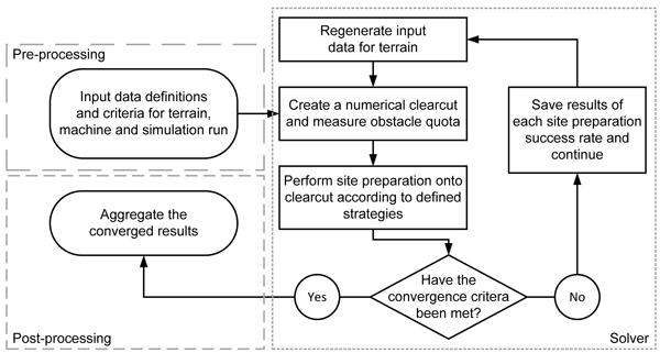
Fig. 1. Flow chart of the conducted simulation following the Monte Carlo method.
Additionally, in order to get information about steady-state conditions that was sought in the simulations, convergence analyses were conducted with respect to some parameters showing significant influence on simulation quality and simulation time. When convergence was found, the parameter could be set accordingly.
2.2 Terrain model
Larsson (2011) acknowledged that failed mounding was caused by subsurface stone and surface boulder occurrence (48%), stump occurrence (34%), slash occurrence (11%) at the mounding site, and other reasons (7%). Lundmark (2006) identified stones, stumps and slash as the critical obstacles during site preparation, while Rantala et al. (2010) emphasized that stones are crucial obstacles that affect mounding efficiency. On that basis stones (both surface and subsurface), stumps and slash were included in the terrain model presented in this paper. Other causes of mounding failure, such as roots interfering with the procedure or lack of mineral soil on the created microsite, were excluded.
2.2.1 Stones and surface boulders
In the terrain model, stones are divided into surface boulders which are visible stones, and subsurface stones. Berg (1982) standardized the technique for measuring the amount of visible stones and stones positioned at a maximum depth of 0.2 m. He divided the amount of surface boulders and subsurface stones into three segments: 25%, 50% and 75% boulder quota. The boulder quota can be estimated by recording the number of times a probe encounters a stone related to the total amount of attempts. The tested terrain model configurations described further in Table 1 have all been tested through Berg’s (1982) boulder quota measuring method in the simulations. Stendahl et al. (2009) showed a correlation between the amount of subsurface stones and surface boulders for moraine soils where a boulder quota of 75% corresponded roughly to 4000 surface boulders per hectare and a 25% boulder quota derived practically no surface boulders at all. Ersson et al. 2014 used a number of 1800 boulders·ha–1 at 55% boulder quota, which was used in our terrain model as well, although transformed into an area percentage number (Table 1) and validated manually.
| Table 1. Five different terrain model configurations based on Ersson et al. (2013) and Berg (1982). Slash residues is further added on these terrain models. | |||||
| Terrain model config. number | Description | Surface boulder amount [Area %] | Stone amount [Area %] | Stump amount [Area %] | Boulder quota |
| 0 | Typical southern Swedish clearcut | 3 | 41 | 4 | ~55% |
| 1 | Few stumps, few stones, no surface boulders. | 0 | 35 | 4 | ~25% |
| 2 | Few stumps, many stones, many surface boulders | 5 | 51 | 4 | ~70% |
| 3 | Many stumps, few stones, no surface boulders | 0 | 35 | 10 | ~25% |
| 4 | Many stumps, many stones, many surface boulders | 5 | 51 | 10 | ~75% |
The size distribution of surface boulders was thoroughly investigated in a study by MarkInfo (2007), which found that a normal distribution of boulder diameters with mean value 0.4901 m and standard deviation of 0.1233 m is a suitable approximation. The normal distribution span was limited to exceed 0.2 m, since smaller diameters were not regarded as surface boulders (MarkInfo 2007). A large common base machine for mounding, Komatsu 865 (Komatsu Forest 2015), has a ground clearance of ~0.7 m. If a surface boulder is assumed to be spherical and its centre is at ground level, the machine operator then needs to avoid boulders with diameter larger than 1.4 m. Therefore, a maximum surface boulder diameter limit of 1.4 m was assumed and the normal distribution span was truncated accordingly.
The subsurface stone sizes followed an exponential distribution (Ersson et al. 2013) with lambda value at 0.05 m, meaning large amounts of small stones and small amounts of rocks larger in size, again assuming a maximum diameter of 1.4 m (i.e. the same as for surface boulders). Andersson et al. (1977) simulated the work operation of mechanized planting units, where stones were included in the terrain model. Here, the minimum size of a cubical stone was set to 50 mm; otherwise, it was not regarded an obstacle. The same conclusions were drawn by Ersson et al. (2013), although a stone was modelled as a sphere with a minimum diameter of 56 mm. In the terrain model used in this study, stones are therefore modelled as circles with a minimum diameter of 56 mm.
2.2.2 Stumps
Herlitz (1975) provided data from 12 stands ready for final felling. In this study, to be able to use a continuous PDF rather than a discrete one for stumps sizes, Herlitz’s (1975) data was approximated by a Rayleigh distribution with Rayleigh parameter 204.755 mm (see Fig. 2). A stump is always surrounded by a root plate; a zone of rapid taper (ZRT), where there is a transition of roots going from the ground which connect to the stump (Wilson 1975). Within this zone, any attempts at mounding usually fail, and this is therefore taken into consideration in the terrain model. Kalliokoski et al. (2008) showed for Fennoscandian species (Betula pendula Roth., Picea abies (L.) Karst. and Pinus sylvestris L.) that the ZRT plus the stump itself (root plate) seldom exceed a diametric plate of 1 m and, furthermore, no significant differences between species could be determined. Therefore, the ZRT was modelled as a constant sized ring outside the stump with a radial size of 0.16 m. The ZRT size was derived from the measure of a ZRT for a mean sized stump (Kalliokoski 2008), where the ZRT size is assumed to be the same for any stump size.
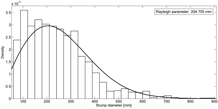
Fig. 2. Stump diameters of 12 stands ready for felling based on Herlitz (1975). The curve represents a Rayleigh distribution with a Rayleigh parameter set to 204.755 mm. The Rayleigh distribution was used to enable the (pseudo)random generator to choose from a continuous domain of values.
2.2.3 Slash
In Sweden, slash is commonly piled and extracted from clearcuts after harvesting (Pettersson and Nordfjell 2007). However, after extraction, remains from such piles form obstacles for subsequent mounding. Pettersson and Nordfjell (2007) measured 552 slash piles where a Swedish, 130-year-old naturally regenerated stand had been clearcut. A layer of 0.2–0.3 m slash remained at such slash pile sites whose size were normally distributed with an average size of 4.06 m2 and 1.4 m standard deviation. In the terrain model, it is assumed that slash only occurs on the clearcut at positions where there are remains from slash piles. Table 2 shows the slash input data for the terrain model. The slash piles were assumed to have a rectangular shape, where we altered the piles length-wise with a fixed width, making the area following a normal probability density function (PDF). The average width-to-length ratio were set to 2:1. The spatial distribution on the clearcut were based on measures from clearcuts of previous spruce stands in southern Sweden where between 200–305 m3sub·ha–1 were harvested (Lars Eliasson, Skogforsk, pers. comm. 2013). The number of slash piles per 100 m strip road were measured, as well as the distance between strip roads (Table 2). We assumed that all terrain model configurations that are used in the simulations have the same slash input data to generate the slash piles.
| Table 2. Slash input data for the terrain model based on Pettersson and Nordfjell (2007) and measures from clearcuts of previous spruce stands in southern Sweden with additional material from Lars Eliasson (Lars Eliasson, Skogforsk, pers. comm. 2013). | |||||
| Distribution type | Mean value | Standard deviation | High limit | Lower limit | |
| Average basal area [m2] | Normal (truncated) | 4.06 | 1.4 | 5.7 | 2.0 |
| Piles per 100 m strip road [-] | Uniform | 8.5 | - | 4 | 13 |
| Distance between strip roads [m] | Uniform | 13.45 | - | 12.5 | 14.4 |
2.2.4 Terrain model configurations
Ersson et al. (2013) proposed different terrain model configurations that are valid for typical Swedish clearcuts. These are used in our simulations (Table 1). Terrain model configuration 0is related to a typical southern Swedish clearcut (Stendahl et al. 2009; Skogsdata 2012), and terrain models 1–4 are chosen in accordance with Ersson et al. (2013) to be able to assess the mounding efficiency for different scenarios.
In addition to the terrain model configurations, slash were determined as described in section 2.2.3, using the same slash input data for all configurations. Berg (1982) suggested a procedure for measuring obstacle occurrence on clearcuts. To retrieve relevant terrain models, this procedure was conducted on clearcuts and iterated until an appropriate boulder quota was found for each terrain model configuration, whereby the area percentage for each object amount was set.
2.2.5 Generating the terrain
All objects in terrain span a 3D space. However, to simplify simulations the objects in the terrain model were projected on a 2D-plane at ground level, i.e. described as pixels in a 2D matrix. Furthermore, the 2D plane does not comprise any height shifts. Thus, some information regarding object size that was described as volumes needed to be transformed into 2D. The value of each element in the 2D matrix was adopted to show the property of it (height, type of object etc.). One parameter states the resolution of the clearcut. For example, a boulder constitutes a circular area on the terrain. That area are built from pixels where a higher resolution allows for a better representation of the sought rounded shape. Thus, a higher resolution (amount of elements in the matrix) give a better representation of the objects, but increase computation time.
An empty terrain model is created onto which objects will be randomly distributed. In addition, each object have specific rules to follow when distributing them in the terrain, e.g. a minimum distance between stumps, no surface boulders lying on top of stumps etc., see Table 3. The amount of each object dispersed onto the terrain is determined by the chosen terrain model configuration (Ersson et al. 2013). It was further assumed that the machine operator is able to avoid objects that could harm the machine or impede accessibility. Therefore, the terrain model excluded any objects that would force the machine to deviate from the route to simplify machine movements.
| Table 3. Object positioning procedure and interrelations between the objects for the creation of the terrain model. | ||||
| Object type (Order of placement) | Boulder (1) | Stump (2) | Stone (3) | Slash (4) |
| Boulder (1) | Can not be placed over top of each other. | Doesn’t exist during boulder placement. | Doesn’t exist during boulder placement. | Doesn’t exist during boulder placement. |
| Stump (2) | ZRT can be placed over top of boulders, not stump. | Can not be inserted closer than 1 metre to another stump (Centre-to-Centre). | Doesn’t exist during stump placement. | Doesn’t exist during stump placement. |
| Stone (3) | Can not be placed under top of boulders. | Can not be placed under the stump centre point | Can not be placed over top of each other. | Doesn’t exist during stone placement. |
| Slash (4) | Can be placed over top of stones. | Can be placed over top of boulders. | Can be placed over top of stumps. | Slash piles never exist in same location. |
The procedure for distributing objects into the terrain model is depicted in Table 3. If the prescribed demands are not met, a new, randomized position is generated for the same object and an identical procedure takes place.
First, surface boulders are randomly distributed, one by one, following a uniform distribution. They can not lie on top of each other. The size of boulders followed a normal distribution (Markinfo 2007).
Second, stumps are distributed on the terrain, one by one. Here, the ZRT of each stump was allowed to be placed over top of boulders and each stump was allowed no closer than one metre to another stump already placed. Stump and ZRT size follow the measurements from Herlitz (1975) (with the size described with a continuous Rayleigh PDF as depicted in Fig. 2) and Kalliokoski et al. (2008) respectively.
Third, sub-surface stones are placed on the terrain, one by one. They are not allowed to be placed under boulders or under the centre point of a stump. In addition, they are not allowed to be placed on top of each other. The size PDF follow an exponential distribution as suggested by Ersson et al. (2013).
Lastly, slash is placed onto the terrain, all piles simultaneously. Here, we chose to simplify the shape of one pile as a rectangle with a width-to-height ratio of 2:1. The scattering of piles and the piles themselves follow Table 2. The angle of the slash piles in relation to the direction of travel of the scarifier is randomly chosen between 0and 90 degrees following a uniform distribution. All piles have the same angle in relation to each other.
2.3 Machine model and terrain relations
It is realistic, even on existing machines, to enable transversal movement (X) and/or enable longitudinal movement of the mounder to somewhat change the mounding site in the direction of travel (Y) (Jukka Alakorpi, Bracke Forest AB, pers. comm. in 2013). Therefore, depending on the movement of the base machine, sites can be chosen in a maximum area of X∙Y metres (area mounding). A longitudinal positioning strategy allows the square area to be chosen anywhere along Y at the mid line, while transversal positioning strategy allows the square area to be chosen anywhere along X at the mid line. With a combined longitudinal and transversal positioning strategy the mounding square area can be chosen anywhere within the X∙Y surface, whereas today’s mounding strategy forces the mound to be created at the midpoint.
To be able to compare transversal and longitudinal movement with each other, X and Y were both chosen at one metre in the simulations. Furthermore, the area X∙Y, representing one microsite, never overlapped another microsite created before or after.
When the terrain has been created, the simulation execution continues with the mounding procedure on the created terrain. The machine travels in a straight line where mounds are conducted with a standard distance length-wise (in all our runs 2 metres) and with 2 metres between each row, in accordance with the specifications of a Bracke M26 mounder. An optimally conducted scarification would these cases result in a mound density of 2500 mounds·ha–1. Mounds are then positioned on the chosen terrain model, where the possibility to change the mound position from the nominal position depends on the positioning strategy. In every mound position the amount of encountered obstacles are measured as the quota of pixels considered obstacles on the intended mound area divided by the number of pixels that compose the entire mound area, while a mean value is derived for the clearcut using quotas from all mounds.
2.4 Simulation quality analysis
Furthermore, to parallelize the simulation code to decrease the total computational time, the mounding was divided into several clearcuts having the same input data. To validate that the results for several runs coincide with results from one long simulation, a test was conducted. Fig. 3 shows the results from one of these runs, where all input data were held constant. A compilation of 5 runs, 75 metres each, were put after each other and compared with one long run of 350 metres. The simulations converged towards the same mean value meaning that it was possible to divide the clearcuts into smaller sections (several short runs compared to one long). Furthermore, as expected when mounding at evenly distributed positions, the cumulative mean value of obstacle amounts within the mounds converged towards the mean value for the entire clearcut terrain model.
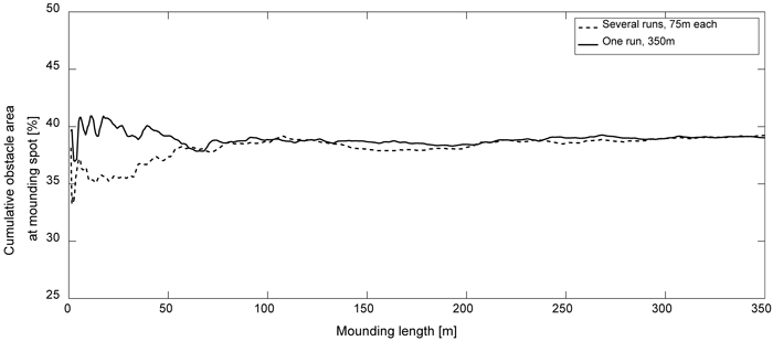
Fig. 3. Graph depicting two runs, one where 5 simulations were run 75 m each and put after one other (dashed line), and one simulation run 350 m (solid line). The simulations converged towards the same cumulative obstacle area at the mounding spots, which occur after around 250 metres.
In order to get information about steady-state conditions, convergence analyses were conducted with respect to clearcut length (fixed width) and clearcut detection resolution, which are two parameters that show significant influence on simulation quality and simulation time. Fig. 3 shows the cumulative mean amount of encountered obstacles at a mound as a function of mounding length (and thus the mounding attempts) with a value of 90 pixels∙m–1 on detection resolution and scarified with one mounding strategy throughout the simulation. From this analysis a minimum 300 m clearcut length was chosen for all simulations in the results section. The detection resolution is also important for the simulation quality and can further be related to needed resolution of any object detection system that could represent a clearcut numerically. Fig. 4 shows the mean obstacle amount as a function of detection resolution with the clearcut length set to 90 m (all other variables are also fixed). From this analysis a resolution of 90 pixels∙m–1 (i.e. ~8100 pixels∙m–2) was chosen for all subsequent simulations.
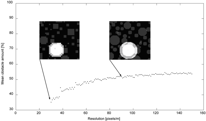
Fig. 4. Simulated mean obstacle amount (area percentage) as a function of detection resolution. A visual representation shows the difference between low-resoluted and high-resoluted clearcuts.
3 Results
Initially, simulations were conducted for each of the three mound positioning strategies (section 2.3) and today’s mounding strategy, applied in each of the five terrain model configurations described in Table 1. To get statistical significance, the clearcuts were each run 75 metres and 10 times (750 metres in total) for every combination of terrain model configuration and positioning strategy. For every re-run, new randomized positions and sizes for objects were used (where the input data for the specific terrain model configuration were fixed). In Fig. 5 the mean obstacle area at the mounding spots are presented for all terrain models 0–4 and for all developed mounding strategies (a low amount of encountered obstacles could imply a better mounding success).
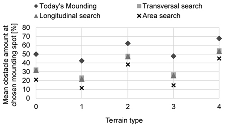
Fig. 5. Mean obstacle area at chosen mounding spots at different terrain models using four different strategies in choosing mounds.
To be able to analyse effects on a larger variation of clearcuts and in this context compare the mound positioning strategies, simulations were conducted where the obstacle quota was changed incrementally (Fig. 6). Mounding was conducted with the four positioning strategies on clearcuts generated in a span from 30% obstacles (which is a lower obstacle quota than used for terrain configuration 1) up to 70% obstacles (which is a higher obstacle quota than used for terrain configuration 4). The obstacle quota was linearly increased from 30% to 70%. In these simulations, the ratio between the different objects was kept constant and could therefore not be entirely compared with the ratios of terrain configurations 0–4.
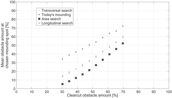
Fig. 6. Mean obstacle amount measured at mounding spots created at clearcuts with total obstacle amounts between 30% and 70%. The obstacles subsurface stones, surface boulders and stumps were linearly changed to range all terrain models 0–4 and more. Slash residue parameters were kept at the same rate throughout the simulations.
4 Discussion
The amount of encountered obstacles using the four compared positioning strategies differs significantly for terrain model configurations 0–4. Today’s strategy encountered on average the same amount as at the clearcut as a whole, longitudinal second-lowest, transversal second-highest and area mounding highest (i.e. the order between the different mounding strategies remains constant, regardless of terrain model). The transversal mounding strategy showed a lower amount of encountered obstacles on average than the longitudinal, possibly since the mounds are modelled as rectangles with the longer side in the longitudinal direction (i.e. requires more space). Hence, since the possibility for transversal and longitudinal movements for the corresponding mounding strategies were set at the same value, it is more likely that successful mounding positions will be found in the transversal direction.
Already at small obstacle quotas, as illustrated in Fig. 5 for terrain model configuration 1, the difference between today’s mounding strategy and the three other suggested mound positioning strategies are significant (around 70% decrease in encountered obstacles). The most notable difference for all mound positioning strategies is caused by a change in subsurface stones (and surface boulders), where the difference between high and low stump quotas is insignificant in comparison to a change in subsurface stones and surface boulders. The difference between today’s mounding procedure and the other suggested procedures is largest at clearcuts with obstacle quotas around 30–50% (where clearcuts having under 30% is unrealistic to encounter). This difference shows that an efficiency improvement potential can be realized by first addressing the need for machine vision, and then the need for new mound positioning strategies that utilise machine vision efficiently.
Today, during operational manual tree planting, trees are typically planted in each mound created by the mounder. If it is assumed that seedlings are planted regardless to whether the created mound was acceptable or not, the seedling survival and growth will be directly related to the result in this paper, showing how mounds created in spots with less amount of obstacles can enable higher seedling survival. In addition, mounding is only used on clearcuts with few obstacles. This result thus shows that on clearcuts with high obstacle quotas, such as terrain configuration 2 and 4 (where mounding is typically not used), mounding can be used since mounds found with better strategies is comparable with mounds found by today’s mounding strategy at much easier clearcuts. Using mounding on more grounds would therefore result in better seedling survival compared to planting on disc-trenched clearcuts (Örlander et al. 1990; Saksa et al. 2005; Uotila et al. 2010). In addition, using more efficient mounding on more clearcut areas in general will render less ground obstruction, possibly lower fuel consumption of the base machine and less wear on the machinery. In fact, some performed site preparations today are of such poor quality that they need to be redone. Therefore, through more efficient mounding procedure, the need to redo the site preparation can be significantly reduced.
The needed resolution of the terrain model described in section 2.4 could be related to the need for a clearcut identification technique to recognize and identify clearcut obstacles, although the resolution need to be interpreted into a 3D representation. The convergence limit of 8100 points∙m–2 chosen for this study can be compared with the Nyquist rate, meaning that at least twice the sampling rate is needed to find the original signal (Nyquist 1928), i.e. a resolution of 8100 points∙m–2 is enough to adequately represent the actual clearcut environment for this purpose, which could be interesting in machine vision aspects to assess the needed quality of the hardware.
Possible limitations in the simulation accuracy can be due to necessary assumptions, e.g. the conversion of some objects’ measurements from 3D to 2D, or the fact that slash was inserted in the same way on all clearcut terrain configurations (although at randomized angles compared to the direction of travel), etc.
Enabling object identification in combination with a mound positioning strategy can significantly improve the mounding success rate and thereby improve subsequent seedling survival while decreasing the environmental impact of site preparation. The potential for machine vision to increase mounding productivity is theoretically high, and we conclude that in this case, it is well worth it to implement remote sensing technologies in silviculture and possibly in forestry as a whole.
Acknowledgements
This work was funded by smart machines and materials, an area of excellence in research and innovation at Luleå University of Technology, and the Swedish research council Formas.
References
Andersson P.-O., Berglund H., Bäckström P.-O. (1977). Simulering av maskinella planteringsorgans arbete. [Simulating the operation of mechanized planting units]. Forskningsstiftelsen Skogsarbeten. Redogörelse nr 7.
Berg S. (1982). Terrängtypschema. [Terrain Classification System for Forestry Work]. Forskningsstiftelsen Skogsarbeten. ISBN 91-7614-078-4.
Ersson B.T., Jundén L., Bergsten U., Servin M. (2012). Simulations of mechanized planting - modelling terrain and crane-mounted planting devices. In: Proceedings of the Nordic Baltic conference on forest operations – OSCAR 2012, Riga, Latvia, October 24–26. Mežzinātne 25(58): 15-18.
Ersson B.T., Jundén L., Bergsten U., Servin M. (2013). Simulated productivity of one- and two-armed tree planting machines. Silva Fennica 47(2) article 958. http://dx.doi.org/10.14214/sf.958.
Ersson B.T., Jundén L., Lindh E.M., Bergsten U. (2014). Simulated productivity of conceptual, multi-headed tree planting devices. International Journal of Forest Engineering 25: 201–213. http://dx.doi.org/10.1080/14942119.2014.972677.
Herlitz A. (1975). Typestands for clear cutting. Royal college of forestry, Garpenberg. Report nr 81. ISSN 0585-332X.
Hussmann S., Ringbeck T., Hagebeuker B. (2008). A performance review of 3D TOF vision systems in comparison to stereo vision systems. In: Bhatti A. (ed.). Stereo vision. p. 103–120. http://dx.doi.org/10.5772/5898.
Jandl R., Lindner M., Vesterdal L., Bauwens B., Baritz R., Hagedorn F., Johnson D.W., Minkkinen K., Byrne K.A. (2007). How strongly can forest management influence soil carbon sequestration? Geoderma 137(3–4): 253–268. http://dx.doi.org/10.1016/j.geoderma.2006.09.003.
Kalliokoski T., Nygren P., Sievänen R. (2008). Coarse root architecture of three boreal tree species growing in mixed stands. Silva Fennica 42(2): 189–210. http://dx.doi.org/10.14214/sf.252.
Kemppainen T., Visala A., (2013) Stereo vision based tree planting spot detection. Robotics and Automation (ICRA), 2013 IEEE International Conference on 6–10 May. p. 739–745. http://dx.doi.org/10.1109/ICRA.2013.6630655.
Komatsu Forest (2014). Komatsu 865. http://www.komatsuforest.us/default.aspx?id=74856&mode=specs&rootID=&productId=74854. [Cited 21 Dec 2015].
Larsson A. (2011). Selection of soil scarification method in northern Sweden within Sveaskog AB domains. Master’s thesis. Swedish University of Agricultural Sciences, Umeå, Sweden. ISSN 1654-1898.
Lideskog H., Ersson B., Bergsten U., Karlberg M. (2014). Determining boreal clearcut object properties and characteristics for identification purposes. Silva Fennica 48(3) article 1136. http://dx.doi.org/10.14214/sf.1136.
Lideskog H., Karlberg M. (2014). Automatic clearcut obstacle identification using a time-of-flight camera. In: Proceedings of the 47th International Symposium on Forestry Mechanization, 23–26 September, Gerardmer, France.
Lundmark J.-E. (2006). Val av markberedningsmetod med hänsyn till markegenskaperna: ståndortsanpassad markberedning. Keynote speech at NSFP days, Tammerfors, Finland.
Luoranen J., Rikala R., Smolander H. (2011). Machine planting of Norway spruce by Bracke and Ecoplanter: an evaluation of soil preparation, planting method and seedling performance. Silva Fennica 45(3): 341–357. http://dx.doi.org/10.14214/sf.107.
Manduchi R., Castano A., Talukder A., Matthies L. (2005). Obstacle detection and terrain classification for autonomous off-road navigation. Autonomous Robots 18(1): 81–102. http://dx.doi.org/10.1023/B:AURO.0000047286.62481.1d.
MarkInfo (2007). Ståndortskarteringen. http://www-markinfo.slu.se/index.html. [Cited 21 Dec 2015].
Metje N., Atkins P.R., Brennan M.J., Chapman D.N., Lim H.M., Machell J., Muggletonc J.M., Pennockf S., Ratcliffed J., Redfernf M., Rogersa C.D.F., Saule A.J., Shanf Q., Swinglerd S., Thomasa A.M. (2007). Mapping the underworld – state-of-the-art review. Tunnelling and Underground Space Technology 22: 568–586. http://dx.doi.org/10.1016/j.tust.2007.04.002.
Metropolis N., Ulam S. (1949). The Monte Carlo method. Journal of the American Statistical Association 44: 335–341. http://dx.doi.org/10.1080/01621459.1949.10483310.
Nyquist H. (1928). Certain topics in telegraph transmission theory. Transactions of the American Institute of Electrical Engineers 47(2): 617–644.
Örlander G., Gemmel P., Hunt J. (1990). Site preparation. A Swedish overview. Chapter 4, site preparation methods. FRDA Report 105.
Petersson M., Örlander G., Nordlander G. (2005). Soil features affecting damage to conifer seedlings by the pine weevil Hylobius abietis. Forestry 78(1): 83–92. http://dx.doi.org/10.1093/forestry/cpi008.
Pettersson M., Nordfjell T. (2007). Fuel quality changes during seasonal storage of compacted logging residues and young trees. Biomass and Bioenergy 31: 782–792. http://dx.doi.org/10.1016/j.biombioe.2007.01.009.
Rantala J., Saarinen, V-M., Hallongren H., (2010). Quality, productivity and costs of spot mounding after slash and stump removal. Scandinavian Journal of Forest Research, 25: 507–560. http://dx.doi.org/10.1080/02827581.2010.522591.
Sabatier J.M. Xiang N. (2001) An investigation of acoustic-to-seismic coupling to detect buried antitank landmines. IEEE Transactions on Geoscience and Remote Sensing 39(6). http://dx.doi.org/10.1109/36.927429.
Saksa T. Heiskanen J. Miina J. Tuomola J., Kolström T. (2005). Multilevel modeling of height growth in young Norway spruce plantations in southern Finland. Silva Fennica 39(1): 143–153. http://dx.doi.org/10.14214/sf.403.
Skogsdata (2012). Forest statistics 2012. Institutionen för skoglig resurshushållning, SLU.
Stendahl J., Lundin L., Nilsson T. (2009). The stone and boulder content of Swedish forest soils. Catena 77(3): 285–291. http://dx.doi.org/10.1016/j.catena.2009.02.011.
Sutton R.F. (1993). Mounding site preparation: a review of European and North American experience. New Forests 7(2): 151–192. http://dx.doi.org/10.1007/BF00034198.
Uotila K., Rantala J., Saksa T., Harstela P. (2010). Effect of soil preparation method on economic result of Norway spruce regeneration chain. Silva Fennica 44(3): 511–524. http://dx.doi.org/10.14214/sf.146.
Wilson B.F. (1975). Distribution of secondary thickening in tree root systems. In: Torrey J.G., Clarkson D.T. (eds.). The development and function of roots. Academic Press, London. p. 197–219.
Total of 32 references.
Send to email
