Adriano Mazziotta  ,
Dmitry Podkopaev,
María Triviño,
Kaisa Miettinen,
Tähti Pohjanmies,
Mikko Mönkkönen
,
Dmitry Podkopaev,
María Triviño,
Kaisa Miettinen,
Tähti Pohjanmies,
Mikko Mönkkönen
Quantifying and resolving conservation conflicts in forest landscapes via multiobjective optimization
Mazziotta A., Podkopaev D., Triviño M., Miettinen K., Pohjanmies T., Mönkkönen M. (2017). Quantifying and resolving conservation conflicts in forest landscapes via multiobjective optimization. Silva Fennica vol. 51 no. 1 article id 1778. https://doi.org/10.14214/sf.1778
Highlights
- We introduce a compatibility index quantifying how targeting a management objective in the forest landscape affects another objective
- To resolve conflicts we find compromise solutions minimizing the maximum deterioration among objectives
- We apply our approach for a case study of forest management for biodiversity conservation and development
- Multiple use management and careful planning can reduce biodiversity conflicts in forest ecosystems.
Abstract
Environmental planning for of the maintenance of different conservation objectives should take into account multiple contrasting criteria based on alternative uses of the landscape. We develop new concepts and approaches to describe and measure conflicts among conservation objectives and for resolving them via multiobjective optimization. To measure conflicts we introduce a compatibility index that quantifies how much targeting a certain conservation objective affects the capacity of the landscape for providing another objective. To resolve such conflicts we find compromise solutions defined in terms of minimax regret, i.e. minimizing the maximum percentage of deterioration among conservation objectives. Finally, we apply our approach for a case study of management for biodiversity conservation and development in a forest landscape. We study conflicts between six different forest species, and we identify management solutions for simultaneously maintaining multiple species’ habitat while obtaining timber harvest revenues. We employ the method for resolving conflicts at a large landscape level across a long 50-years forest planning horizon. Our multiobjective approach can be an instrument for guiding hard choices in the conservation-development nexus with a perspective of developing decision support tools for land use planning. In our case study multiple use management and careful landscape level planning using our approach can reduce conflicts among biodiversity objectives and offer room for synergies in forest ecosystems.
Keywords
biodiversity;
ecosystem management;
forestry;
decision support tools;
environmental conflicts;
land-use planning;
systematic conservation planning
-
Mazziotta,
University of Jyväskylä, Department of Biological and Environmental Science, P.O. Box 35, FI-40014 University of Jyväskylä, Finland; Center for Macroecology Evolution and Climate, University of Copenhagen, Universitetsparken 15, DK-2100 Copenhagen, Denmark; Stockholm Resilience Centre, Stockholm University, Kräftriket 2b, 11429 Stockholm, Sweden
 http://orcid.org/0000-0003-2088-3798
E-mail
a_mazziotta@hotmail.com
http://orcid.org/0000-0003-2088-3798
E-mail
a_mazziotta@hotmail.com
- Podkopaev, University of Jyväskylä, Department of Biological and Environmental Science, P.O. Box 35, FI-40014 University of Jyväskylä, Finland; Systems Research Institute, Polish Academy of Sciences, Newelska 6, 01-447 Warsaw, Poland E-mail dmitry.podkopaev@ibspan.waw.pl
- Triviño, University of Jyväskylä, Department of Biological and Environmental Science, P.O. Box 35, FI-40014 University of Jyväskylä, Finland E-mail maria.trivino@jyu.fi
- Miettinen, University of Jyväskylä, Faculty of Information Technology, P.O. Box 35, FI-40014 University of Jyväskylä, Finland E-mail kaisa.miettinen@jyu.fi
- Pohjanmies, University of Jyväskylä, Department of Biological and Environmental Science, P.O. Box 35, FI-40014 University of Jyväskylä, Finland E-mail tahti.t.pohjanmies@jyu.fi
- Mönkkönen, University of Jyväskylä, Department of Biological and Environmental Science, P.O. Box 35, FI-40014 University of Jyväskylä, Finland E-mail mikko.monkkonen@jyu.fi
Received 11 January 2017 Accepted 23 January 2017 Published 2 February 2017
Views 161265
Available at https://doi.org/10.14214/sf.1778 | Download PDF

Supplementary Files
1 Introduction
Biodiversity can be considered a multi-faceted phenomenon including taxonomic, phylogenetic and functional species diversity as well as population’s genetic diversity and variation among ecosystems (MEA 2005). This creates a challenge for planning any actions or making management decisions that aim at securing or protecting biodiversity. As a complex concept, biodiversity can be measured in a variety of ways (Magurran 2004), and consequently managers need to select which objectives or measures of biodiversity they will focus on.
As different biodiversity objectives (i.e. species in our case study) are often antithetical or conflicting, management actions for one objective can be detrimental to achieving other objectives (Prendergast et al. 1993; Similä et al. 2006; Kahilainen et al. 2014). In other words, there may be conflicts between management plans designed to conserve different biodiversity objectives, and no single management action is beneficial for biodiversity as a whole. A multispecies approach for conservation must reflect the spatial, compositional and functional complementarity of the biodiversity objectives. It has been suggested that this approach should be based either on the selection for protection of several “focal” species or on “landscape” species, as well as on their response to human-induced threats (Lambeck 1997; Sanderson et al. 2002). However, setting priorities on the basis of the requirements of selected species can be biased by incomplete data (Lindenmayer et al. 2002). Moreover, prioritization among biodiversity objectives should not consider only species’ biological value and vulnerability (i.e. their threat status), but also other aspects including their economic, social and cultural values and practical issues such as feasibility of conservation actions (Mace et al. 2007; Joseph et al. 2009). In this respect, management planning for the persistence of different biodiversity aspects should consider multiple contrasting objectives based on alternative uses of the landscape (Redpath et al. 2013).
In the classical prioritization approach to conservation planning, units of a landscape are preferentially associated to different uses by ranking them for their ecological/economic value. Species richness has been used as a short-cut to overall biodiversity value and a target to be maximized (for a review, see Cullen 2013). However, species richness may be a problematic objective because components of biodiversity that require conservation do not necessarily co-occur within biodiversity hotspots (Prendergast et al. 1993; Similä et al. 2006). Ecological value of the landscape elements has also been defined and weighted by their capacity to support multiple biodiversity objectives such as multiple threatened or indicator species or their habitats. Economic weights are typically attributed to the landscape units on the basis of their capacity to produce revenues. However, the attribution of ecological and economic weights to the landscape units can be seriously biased. Weights are often subjective and static, incapable of addressing the dynamics in ecological and economic systems (for difficulties and shortcomings of expressing relative importance with weights, see, e.g. Roy and Mousseau 1996; Nakayama 1997). For example, occurrence and abundance of species and their habitats can be dynamic across space and time, and their weights should vary accordingly. Economic weights are well defined once parameters like land productivity are defined, but also economic values change over time e.g. according to societal demand and variability in land productivity.
As an alternative to the classical weight-based prioritization, we introduce an approach to allocate different management regimes to landscape elements while simultaneously maximizing habitat availability for different biodiversity objectives in the landscape, solving the conflicts among them, and also considering an economic constraint. This comprehensive approach to conservation planning reduces trade-offs in the landscape. The simultaneous maximization approach attributes all the landscape elements to different land uses for simultaneously targeting multiple ecological and economic goals in the landscape. In this case, landscape units are not dedicated to pursue either an ecological or an economic objective, like in the classical prioritization approach, but they all contribute to reduce trade-offs between ecological and economic objectives.
In dynamic forest ecosystems, conservation prioritization based on static weights is problematic because the ecological value of each forest patch varies in time as a function of natural and human-induced disturbances. Forests are important sources of goods and services for the society. Boreal forests, for example, provide approximately 45% of the world’s stock of growing timber, and about one-quarter of the global exports of forest industry products (IUFRO 2012). These forests comprise about one third of the global carbon storage and one fifth of the global carbon sinks in forests (Pan et al. 2011). In Fennoscandia, the majority of land area is covered by forests and most of them are intensively managed for timber production. Intensive management is the main cause of loss of biodiversity in the Nordic boreal forests (Mönkkönen 1999). Nevertheless, it has been shown that in boreal landscapes small changes in management can support biodiversity elements (single species and species groups) with small losses in timber revenues (Mönkkönen et al. 2014). Therefore, it is important to develop tools which maximize the landscape capacity to support biodiversity while limiting the economic losses.
In this study, we first develop an approach to describe and measure conflicts among different biodiversity objectives on the basis of the capacity of the landscape to simultaneously sustain them. We then propose an approach to resolve these conflicts through landscape level management planning. Finally, we present a case study in a boreal forest landscape to verify the potential utility of this approach. The aim of the case study is finding a management plan that minimizes conflicts among ecological (species) and economic (timber production) objectives. Here we use the maximization of habitat availability as biodiversity objective for a set of umbrella species. We employ the approach for solving conflicts at a large landscape level across a long 50-years planning horizon. A large spatial extent is necessary to retain the overall quality of the landscape in dynamic forest ecosystems, where the quality (as species habitat or timber revenue) of individual land units may vary dramatically over time. Likewise, a long-term focus is a prerequisite because today’s land use and land management decisions have far reaching consequences that may realize after long time lags. This is particularly evident in forest ecosystems where a rotation typically lasts for decades.
2 Materials and methods
2.1 The multiobjective optimization problem of targeting biodiversity
When making management plans for a given landscape, alternative objectives of biodiversity play the role of objective functions and as said, they typically are conflicting. We formulate the planning problem as a general multiobjective optimization problem using the terminology of Miettinen (1999). The problem is to find a management plan x among the given set of possible plans, which maximizes the vector of outcomes in terms of given biodiversity objectives:

where X is the set of all possible management plans called feasible solutions; k is the number of biodiversity objectives; f1, f2,…,fk are real-valued objective functions, where fk(x) evaluates the management plan x in terms of the k-th objective. The vector (f1(x), f2(x), …, fk(x)) is called the outcome of plan x.
It is unlikely that for a real-life problem formulated as (1), there exists a solution maximizing all objective functions simultaneously. Indeed, if a management plan results in the highest possible value for some biodiversity objective in the given landscape, the results for other objectives may be far from optimal. Therefore, instead of searching for a solution that is optimal with respect to all objectives simultaneously, in multiobjective optimization so-called Pareto optimal solutions are considered (Miettinen 1999). A solution is Pareto optimal if it cannot be improved with respect to any objective without causing losses in at least one of the other objectives. The existence of (usually, multiple) Pareto optimal solutions is guaranteed under weak mathematical conditions, naturally satisfied in most of practical problems including ours. Thus, in practice, we deal with different Pareto optimal solutions involving different trade-offs.
Obviously, it is not worth implementing a plan if it is not Pareto optimal, because another plan exists providing a better outcome. Therefore, solving a multiobjective optimization problem is understood as finding the Pareto optimal solution that is the most preferred for a decision maker, or in its absence, deriving the set of all Pareto optimal solutions or a representative subset of them (whenever deriving the whole set is not possible). Here, a decision maker refers to a forest owner who can provide preference information related to different solutions and objectives.
Many approaches to conservation planning can be framed as multiobjective optimization problems. For example, the most popular software framework Marxan (Ball and Possingham 2000) solves optimization problems where multiple conservation targets can be framed as additional constraints. In such problems, one of the conservation targets is selected to be the optimization objective while the rest are constraints (in each constraint, the conservation target plays the role of the left-hand side and the bound plays the role of the right-hand side). By varying these targets, one can obtain different Pareto optimal solutions of the problem where these features play role of different objectives. Another popular method (Moilanen et al. 2005; Lehtomaki and Moilanen 2013), implemented as the famous Zonation software, produces series of spatial prioritization solutions which can be interpreted as trade-off curves. Unlike other approaches, we use multiobjective optimization not for making conservation planning decisions but for analyzing the complex set of Pareto optimal possibilities existing in the management of a landscape. In other words, unlike the other two software we build a graph of conflicts and propose here a way of resolving conflicts. Our method is not an alternative way for solving conservation planning problems but to define and resolve conservation conflicts.
2.2 Quantifying conflicts between biodiversity objectives
The notion of conflict occurs when comparing different Pareto optimal solutions, for which improving one objective can be achieved only at the expense of other objective(s). Here, in order to quantify the conflicts between two biodiversity objectives, denoted by objectives 1 and 2 (i.e., f1 and f2), we consider the set of Pareto optimal solutions of the bi-objective optimization problem where only these two objectives are taken into account:

In this case, the set of Pareto optimal solutions can be visualized as a curve representing different trade-offs, that is, a so-called trade-off curve (Fig. 1).
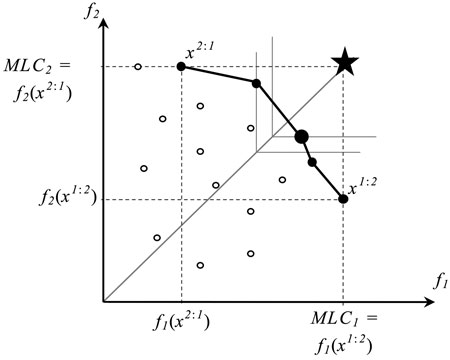
Fig. 1. A set of outcomes of feasible (○) and Pareto optimal solutions (●) of a bi-objective optimization problem. The horizontal (f1) and vertical (f2) axes correspond to biodiversity objectives 1 and 2, respectively, and x2:1 and x1:2 refer to extreme solutions corresponding to values of Maximum Landscape Capacity (MLC) (i.e., Pareto optimal outcomes). The large dot represents the Pareto optimal solution (management plan) that is closest to the ideal plan (star) where all objectives reach their maximal values. The solutions´ points are connected for visualization purposes only.
Let us consider the two extreme points, along the trade-off curve corresponding to the two Pareto optimal solutions, which individually maximize values of the two objective functions respectively (Fig. 1). For f1, by solving the single-objective optimization problem:

we can find the highest value of the f1 achievable in the landscape by any feasible management plan. We call this value the maximum landscape capacity of f1 (MLC1). The value of MLC2 is calculated correspondingly. It is important to note that a plan maximizing a given objective function is not necessarily unique. For example in Fig. 1, there are two solutions (a feasible solution and a Pareto optimal one) having the value of f2 objective function equal to MLC2.
Among the set of all plans that maximize f1, we select a plan which has the maximum value of f2. This plan is denoted by x1:2. It can be formalized as the solution to the following problem:
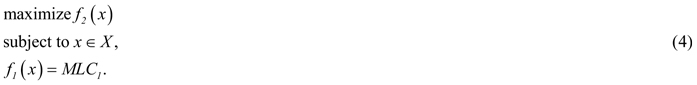
Observe that x1:2 is one of the two extreme solutions introduced in Fig. 1: its outcome (f1(x1:2), f2(x1:2)) represents the Pareto optimal solution with the highest possible value of f1 and the smallest value of f2 (among Pareto optimal solutions). The other extreme solution x2:1 is obtained in an analogous way.
The percentage ratio between f2(x1:2) and MLC2 shows how much maximizing f1 affects the capacity of the landscape for providing f2. We call this ratio compatibility index of objective 1 to objective 2 and denote it by R1(2):

High values (close to 100%) of the compatibility index mean that the biodiversity objective 1 is compatible with the biodiversity objective 2, i.e., improving objective 1 does not significantly affect the possibility to achieve high values of objective 2.
2.3 Resolving conflicts
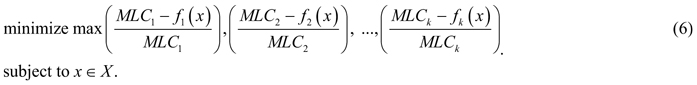
As argued above, it is unlikely to find a management plan that would simultaneously provide maximum values for all the biodiversity objectives; however, there are Pareto optimal management plans that can be considered as candidates for the problem solution. According to the Pareto optimality principle, improving one biodiversity objective relates to deterioration of some others, which is referred to as a conflict between objectives. Resolving such a conflict can be understood as finding a Pareto optimal solution whose outcome represents a “good compromise” between values of different objectives. The notion of “good compromise” cannot be defined mathematically, but should be related to preferences of the decision maker (in our case – the forest owner). In the absence of communication with the owner of the considered landscape, we construct the model of decision maker’s preferences based on the general, rational principle of minimax regret (Savage 1951). A decision maker following the minimax regret strategy aims at minimizing very large opportunity losses from having made the wrong decision, i.e. avoid the highest risks. We hypothesize that a rational decision maker can base his/her preferences on this widely known principle, and therefore applying the constructed preference model represents a realistic decision making scenario. The minimax regret principle in our framework of multiobjective optimization can be formulated as follows (see, e.g., Yu 1973, and Zeleny 1982): find a Pareto optimal solution whose maximum (among objectives) relative deterioration of objective function value with respect to the corresponding MLC is minimal (among all Pareto optimal outcomes). For a problem (1) with k objectives, such a compromise solution can be obtained by solving the following optimization problem:
All variables are positive and measured in a relational scale. Note that the solution to the problem (6) may be not Pareto optimal, but weakly Pareto optimal, meaning that it can be improved in some (but not all) objectives simultaneously without deterioration of the other objectives. Therefore, special techniques are used for ensuring Pareto optimality in problems like (6) (Miettinen, 1999). In our calculations presented in this paper, we apply the ε-constraint method consisting of the following: after the solution to problem (6) is obtained with the outcome denoted by y͂ = (y͂1, y͂2,..., y͂k), for each objective i subsequently from 1 to k we solve the problem:
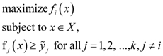
and replace ỹ1 with the optimal value of the latter problem. The solution to the last problem (when i = k) will be a Pareto optimal solution of problem (6).
The elements of maximum in formula (6) represent the set of percentage losses of the objective function values relative to their maximal values (MLC). Thus, the combined objective function of (6) evaluates plans according to the maximum relative deterioration among objectives comparing to their maxima, and seeks for a plan whose maximum relative deterioration is as small as possible. In other words, we try to minimize the distance of a management plan to the ideal point that has maximum objective function values as its components.
For a bi-objective problem, this compromise solution is illustrated in Fig. 1 as a large black dot, where the star represents the ideal point and thin lines refer to the level curves of the objective function (6). The level curves in the case of two objectives are pairs of orthogonal half-lines, which originate from the reference line connecting the origin and the ideal points (shown by a solid grey line). Moving the level curve along the reference line a Pareto optimal solution can be found that solves the optimization problem (6). Such an approach is popular in multiple criteria decision making in cases where no information about decision maker’s preferences is available (see e.g. Miettinen 1999).
Our approach can be summarized as follows (see the scheme in Supplementary file S1, paragraph 1). In order to evaluate the intensity of conflict between two biodiversity objectives (denoted by objectives 1 and 2), we solve problem (3) for each of the objectives in order to find MLC1 and MLC2. Then for each of the objectives, we solve problem (4) in order to find extreme solutions x1:2 and x2:1. The intensity of the conflict between objectives 1 and 2 is evaluated by compatibility indices R1(2) and R2(1) calculated using formula (5). In order to resolve the conflict between a given set of objectives (e.g., all the objectives or a pair of them), we obtain a management plan which minimizes the maximum (among objectives) relative deterioration with respect to their MLC by calculating a Pareto optimal solution of problem (6), formulated for the considered set of objectives.
2.4 Case study
Our study area is a typical boreal production forest landscape located in South Central Finland (62°14´N, 25°43´E). The total area is 687 km2 of which forest on mineral soils covers 55%, peat lands 13%, lakes 16% and farmland settlement some 15% of the area. The dominant tree species are Scots pine (Pinus sylvestris L.), Norway spruce (Picea abies (L.) H. Karst.) and birch (Betula pendula Roth and Betula pubescens Ehrh.).
We obtained raw forest data from the Finnish Forest Centre (http://www.metsakeskus.fi/), an administrative unit for forest management, and the output data from the MOTTI forest growth simulator belong to the Natural Resources Institute of Finland (https://www.luke.fi/en/). The data are organized as forest stands that are basic units for forest inventories. The landscape consists of 29 706 stands with an average size of 1.45 hectares (stand size ranges between 0.06 and 17.5 hectares). We considered seven alternative management regimes for each stand, varying between the recommended intensive management (Yrjölä 2002) and total protection. For further details, see the management regimes in Table 1, and Mönkkönen et al. (2014) and Triviño et al. (2015).
| Table 1. Management regimes applied on the forest stands (modified from Triviño et al. 2015). | ||
| Management regime | Acronym | Description |
| Business as usual | BAU | Recommended management: average rotation length 80 years; site preparation, planting or seedling trees; 1–3 thinnings; final harvest with green tree retention level 5 trees ha–1 |
| Set aside | SA | No management |
| Extended rotation (10 years) | EXT10 | BAU with postponed final harvesting by 10 years; average rotation length 90 years |
| Extended rotation (30 years) | EXT30 | BAU with postponed final harvesting by >30 years; average rotation length 115 years |
| Green tree retention | GTR30 | BAU with 30 green trees retained/ha at final harvest; average rotation length 80 years |
| No thinnings (final harvest threshold values as in BAU) | NTLR | Otherwise BAU regime but no thinnings; therefore trees grow more slowly and final harvest is delayed; average rotation length 86 years |
| No thinnings (minimum final harvest threshold values) | NTSR | Otherwise BAU regime but no thinnings; final harvest adjusted so that rotation does not prolong: average rotation length 77 years |
We ran forest growth simulations for 50 years in 5-year intervals, that is, 11 time steps. The development of forest stands under different management regimes was modeled using the MOTTI stand simulator (http://www.metla.fi/metinfo/motti/index-en.htm). MOTTI is based on statistical tree growth and yield models and describes the effects of management on tree growth. The output variables from MOTTI are time series for tree regeneration, growth, and mortality. The estimates of tree growth and mortality produced by MOTTI become less reliable the more mature the forest is (e.g., Holopainen et al. 2010). However, this time window is longer than the typical forest planning horizon of 10–20 years (http://www.fao.org/docrep/w8212e/w8212e07.htm) and conveniently short to allow us not to take into account the effects of climate change on forest growth, which will become more evident towards the end of the 21st century (Kellomäki et al. 2008).
We evaluated conflicts among six focal species (biodiversity objectives): capercaillie (Tetrao urogallus L.), flying squirrel (Pteromys volans (L.)), hazel grouse (Bonasa bonasia (L.)), long-tailed tit (Aegithalos caudatus (L.)), lesser-spotted woodpecker (Dendrocopos minor (L.)) and three-toed woodpecker (Picoides tridactylus (L.)). These species represent a wide spectrum of habitat associations, responses to management actions, and conservation and societal values (Mönkkönen et al. 2014). We extracted forest stand characteristics from MOTTI simulation outputs and translated them into Habitat Availability using species-specific sub-utility functions. Habitat availability is dynamic through time as a function of the management regime applied in the habitat and the associated forest growth. We calculated average habitat availability indices across 50 years as proxies for species population sizes. For more details on the calculation of the habitat availability for each species, see Mönkkönen et al. (2014) and Suppl. file S1 (in paragraph 3: “Species and their habitat availability”).
In order to transform the extracted timber into an economic value, we calculated the net present value (NPV) of harvest revenues, after 50 years, for each management regime and forest stand. In these calculations, we used stumpage prices for eight timber assortments (pulp wood and saw logs for each tree species: Scots pine, Norway spruce and two birch species) and unit costs of five different silvicultural work components including natural regeneration, seedling, planting, tending of seeding stands, and cleaning of sapling stands (Finnish Statistical Yearbook of Forestry 2011). The average amounts of harvested pulp wood and saw log from thinnings and final harvest under alternative management regimes are the same as in Fig. S2 in Peura et al. (2016). In addition, we applied a 3% real interest rate in discounting the revenues and costs occurring at different time periods. For further details, see Mönkkönen et al. (2014). The choice of an appropriate discount rate when estimating net present value is a controversial and critical issue, especially for studies involving long time horizons. However, for forestry, investments are typically bigger than 2% (e.g., Grege-Staltmane and Tuherm 2010). In other studies examining trade-offs between conservation and economic-objectives the shapes of the Pareto-frontiers were similar under 1–10% discount rate scenarios, while the absolute values varied (Cheung and Sumaila 2008). Different market prizes for the timber could also influence the identified trade-offs.
In the multiobjective optimization problem of forest management planning formulated as (1), each feasible solution (a forest management plan) is defined via a matrix x = (xsp)m×n ∈ {0,1}m×n, where rows correspond to stands (s ∈ {1, 2,…, m}, m = 29 706) and columns correspond to management regimes (p ∈ {1, 2,…, n}, n = 7). This matrix defines the assignment of management regimes to stands as follows: the element xsp at the s-th row and the p-th column takes the value 1 if regime p is applied to stand s and xsp is 0otherwise. Each stand can be assigned with one regime and, therefore, the sum of elements of each row should be equal to one. Thus, the feasible solution set is defined by:
![]()
In order to define objective functions, for each forest stand s, management regime p and species q = 1, 2,…,k with k = 6, we denote by ![]() the habitat availability of the forest stand s for species q resulted from applying the p-th management regime. The habitat availability value of the landscape is defined as the sum of habitat availability values for all stands and, therefore the objective functions are formulated as:
the habitat availability of the forest stand s for species q resulted from applying the p-th management regime. The habitat availability value of the landscape is defined as the sum of habitat availability values for all stands and, therefore the objective functions are formulated as:
![]()
In order to solve optimization problems (3), (4) and (6) where the set of feasible solutions and the objective functions are defined via (7) and (8) respectively, one can use Marxan with Zones (Watts et al. 2009) which also employs an equivalent of the ε-constraint method. In terms of Marxan´s mathematical model, the management regimes can be interpreted as zones a forest stand can be allocated to; negated habitat availability values of forest stands as costs; and the right-hand sides of constraints as targets for conservation features. Observe that Marxan uses simulated annealing algorithm for obtaining approximate solutions of such problems in the case of high computational complexity. In our case study, it was enough to use IBM’s CPLEX Optimizer™ that provided exact solutions to all Mixed-Integer Linear Programming (MILP) problems we needed to solve, including problem (6) reduced to MILP using the ε-constraint method.
3 Results
We found a high median value of the compatibility indices (90%) among the six species (considering all the possible pairwise solutions maximizing landscape capacity for single species), an indication of a small overall conflict among species’ habitat availability (Fig. 2). However, the compatibility index varied widely between 46% and 99.7% (grey boxplots in Fig. 2, all the pairwise Pareto optimal solutions for the compatibility indices are reported in Table S2 in Suppl. file S1, paragraph 2: “Compatibility indices and proportions of management options”). While some species were more compatible with all the others, i.e., maximizing their habitat availability would not considerably reduce habitat availability for the other species, some species revealed both high and low levels of conflicts. The most compatible species were the capercaillie and the lesser spotted woodpecker, which showed high median compatibility index values with all the other species (Fig. 2). The other four species showed both high and low conflict levels. The hazel grouse had compatibility index values consistently below the median of the extreme solutions (Fig. 2).
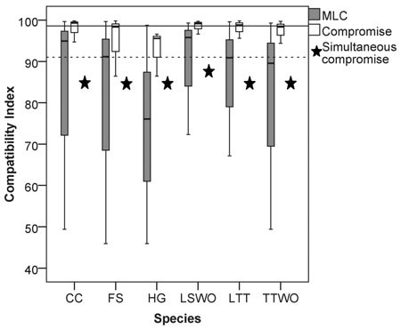
Fig. 2. Box (median and interquartile range) and whiskers (variability outside quartiles) plots show the range of compatibility index values for each species for: (grey) pairwise solutions maximizing landscape capacity for a single species (MLC), and (white) pairwise compromise solutions. Stars represent relative habitat availability under a compromise solution that simultaneously minimizes the loss of habitat for all the species, expressed in terms of % of habitat availability to MLC. The horizontal reference lines represent the median value among all the species for: (dotted line) solutions maximizing single-species landscape capacity and (continuous line) the pairwise compromise solutions. Abbreviations on the x-axis: CC = capercaillie, FS = flying squirrel, HG = hazel grouse, LTT = long-tailed tit, LSWO = lesser-spotted woodpecker, TTWO = three-toed woodpecker.
We found that the compatibility index is asymmetric. This means that maximizing habitat availability for species 1 affects the capacity of the landscape to provide habitat for species 2 in a different way compared how maximizing habitat availability for species 2 affects species 1 (Fig. 2, Table S2). For example, maximizing habitat availability for the hazel grouse (HG) was in strong conflict (RHG(FS) = 45.9%) with maximizing habitat for flying squirrel (FS), while maximizing habitat availability for flying squirrel resulted in a much smaller conflict (RFS(HG) = 74.4%) with habitat for hazel grouse (Table S2, Fig. 3). The asymmetry of the compatibility index can be explained by the fact that each species achieves the maximal habitat availability through a species-specific combination of management regimes across the stands, which does not depend on the combination of management regimes maximizing habitat availability for other species. The management plan maximizing habitat for a certain species modifies the capacity of the landscape to provide habitat for other species in a unique way, thus switching the role of species when calculating the compatibility index between them does not lead to the same result.
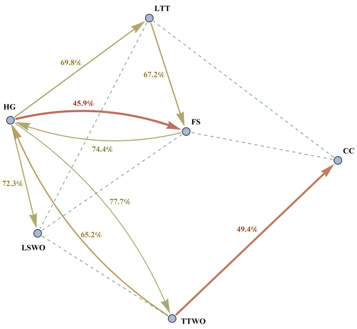
Fig. 3. Graph of compatibility indices R1(2) and R2(1) between different pairs of species. The figure shows conflicts between species as follows: an arrow from species 1 to species 2 represents the level of compatibility of the species 1 to the species 2. More intense conflicts (lower compatibility indices) are represented by thick red arrows, intermediate conflicts by thinner yellow arrows. Only conflicts with the compatibility index less than 85% are shown for better readability. Dashed lines are drawn between pairs of species which have high reciprocal compatibility index values (for which R1(2) + R2(1) ≥ 190%). Species abbreviations are as in the caption of Fig. 2.
In order to obtain management plans, which provide compromise habitat availability values resolving the conflicts for each pair of species, we solved problem (6) with k = 2 (range of solutions in the white boxplots in Fig. 2, Table S2). Here and henceforth, solution of problems formulated as (6) using the ε-constraint method was reduced to solving mixed-integer linear programming problems, which in its turn were solved by using IBM’s CPLEX Optimizer™. The median values of the compromise solutions were always higher than the median values of the pairwise solutions for species compatibility indices (cf. grey and white boxplots in Fig. 2, Table S2) indicating that in all cases the pairwise compromise solution moderated the conflict for both species. In general, the median value of the compatibility indices for compromise solutions (99%) was about 8% higher than the median value of the solutions maximizing landscape capacity for single species (Fig. 2, Table S2). There was, however, much variation in how large the relative improvements were when compared to the pairwise solutions maximizing landscape capacity for single species. For example, in the case of the strong asymmetric conflict between the hazel grouse and the flying squirrel (Fig. 3, Table S2), the compromise solution resulted in a higher proportion of available habitat for the two species (86% of the maxima) than was achieved without simultaneous consideration of habitat availability. This benefit was higher for the hazel grouse (41% improvement with respect to the average of the pairwise solutions maximizing its landscape capacity) than for the flying squirrel (12% improvement) (Fig. 2, Table S2).
Such important improvements in habitat availability through compromise solutions can be explained by the underlying asymmetry in their conflicts and the shapes of pairwise trade-off curves. Moving away from a solution maximizing landscape capacity only for one species (open circles in Fig. 4) towards compromise solutions (black dots), one species receives significant improvement of habitat availability at the expense of relatively small deterioration of the other species’ habitat availability (Fig. 4). For example, the management plan achieving compromise solution between flying squirrel and hazel grouse increased habitat availability for both the species respect to the plans alternatively maximizing habitat for one of them. Flying squirrel had an average increment in habitat availability of 0.36 (SD = 0.31) for 18.3% of the plots, while hazel grouse had an average increment in habitat availability of 0.23 (SD = 0.13) for 8.5% of the plots (Fig. 5). From the comparison of spatial maps of the three management plans (Fig. 5), it is evident that assignment of management regimes sharing habitat fairly between two species (green areas) does not significantly change and is present in both management plans when one species is targeted. On the other hand, there are many areas switching between management regimes beneficial for one of the species (Fig. 5). Thus, when targeting more than one species, one cannot achieve efficient (Pareto optimal) outcomes by using only land sparing strategy.
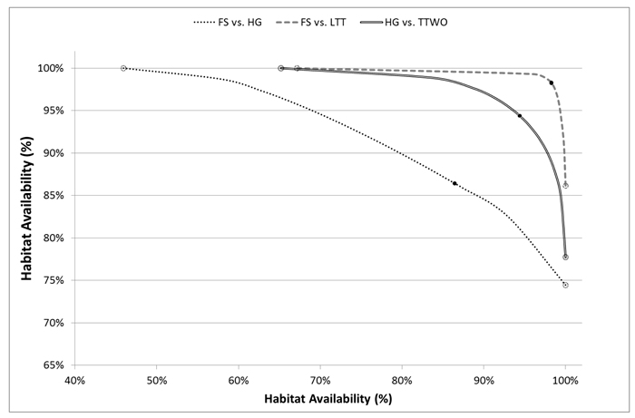
Fig. 4. Trade-off curves for habitat availability of selected pairs of species for which at least one conflict is evident (one of the two compatibility indices is low) plotted in x and y-axes. Solutions deriving from management plans maximizing landscape capacity for single species are pointed out on the curve with empty dots, compromise solutions with black dots. Species abbreviations are in the caption of Fig. 2.
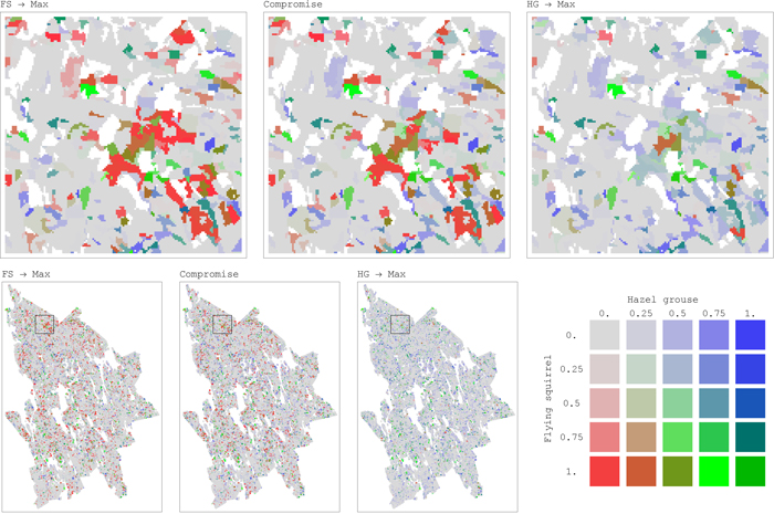
Fig. 5. Maps of distribution of habitat availability values for a pair of conflicting species, flying squirrel (FS) and hazel grouse (HG), in the study area for each forest stand (25 m × 25 m resolution) (maps on top present magnification of regions, outlined in the map at the bottom left with black square borders). Habitat Availability combinations for the two species shown in each of the three maps represent outcomes of the corresponding management plans: maximizing landscape capacity for one species only (FS → Max, HG → Max) and the compromise management plans addressing landscape capacity for both the species. The color palette is defined by the ratio between habitat availability values of the two species. The intensity of the color corresponds to the absolute values of habitat availability. Color legend: red when habitat availability of FS is positive while habitat availability of HG is zero. Blue when habitat availability of HG is positive while habitat availability of FS is zero. Green when both species’ habitat availabilities are positive and “fairly” shared between them. The “fair” share is defined as the ratio between the average values of maximum (across management regimes) habitat availability achieved for each species at each stand, where only positive habitat availability values are considered, for FS and HG these averages are 0.42 and 0.32, respectively. View larger in new window/tab
When solving problem (6) involving all six species, we obtained a management plan that provided for each species at least 85% of its Maximum Landscape Capacity (stars in Fig. 2). This simultaneous compromise solution provided lower median habitat availability than the pairwise compromise solutions (white boxplots in Fig. 2). The simultaneous compromise solution also resulted in lower habitat availability than the median of the pairwise solutions for all other species except the hazel grouse. This is the price one has to pay when optimizing several objectives at the same time. The benefit of doing so is the marked reduction in the variation among single species solutions (Fig. 2).
Economic costs should be integrated in conservation planning (Naidoo et al. 2006). As timber is the main commercial good from production forests, management plans aiming to target biodiversity should also take into account economic returns from timber extraction. The maximum timber NPV that can be obtained from the landscape considered is 250 M€ across the 50 year planning period (average 5800 € ha–1), consisting mainly of the business as usual (BAU > 60% of the stands) and no-thinnings short rotation regimes (NTSR≈10%), while the NPV corresponding to the simultaneous compromise solution of the problem (6) provides 126.9 M€ where in half of the stands NTRS is applied, and BAU management is halved (≈30%). Details on the share of management options applied for the three scenarios are provided in Suppl. file S1 in Figure S1 (paragraph 2: “Compatibility indices and proportions of management options”). Thus, reaching the level of at least 85% of MLC for the six species approximately halved the maximum timber NPV. This is a consequence of the conflict between timber harvesting and species habitat availability showed by Mönkkönen et al. (2014).
In order to make the management plan that resolves the conflict between species acceptable by forest managers and owners, we introduced into the optimization problem (6) an economic constraint: NPV from timber extraction should account 95% of its maximal possible level. The level of 5% reduction in NPV was selected because it roughly corresponds to the amount of money the society would forego to improve habitat for biodiversity, which is in agreement with the political decisions already taken in Finland regarding biodiversity conservation through the METSO II program (Finnish Forest Research Institute 2012). Because of the 95% NPV economic constraint, habitat availability of all species relative to MLC dropped considerably below the levels in the simultaneous compromise solution without the constraint (Fig. 6). There was variation among species in the reduction. The smallest reduction resulting from introducing the constraint was 13% (for the hazel grouse) and the largest was 29% (for the flying squirrel). In this case, the management plan was dominated by NTSR (50% of the stands) and by a smaller quote of stands was set-aside (SA≈10%) (Fig. S1).
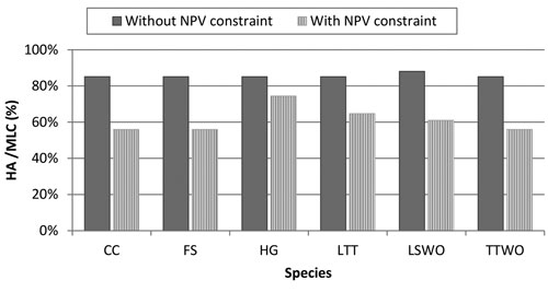
Fig. 6. Comparison of simultaneous compromise solutions for all the six species without and with money constraint. The simultaneous compromise solutions, expressed in terms of percentage Habitat Availability (HA) to Maximum Landscape Capacity (MLC), minimize the loss of habitat among all the species. The management plan obtained by the solution without NPV (Net Present Value) constraint aims at only solving conflicts among all species, the management plan with NPV constraint solves conflicts among all species while obtaining 95% of the NPV from timber extraction. Species abbreviations are in the caption of Fig. 2.
4 Discussion
In this study we addressed a recurring problem in conservation biology: if a management plan is focused just on a single biodiversity objective, the landscape loses its potential for achieving other objectives. We addressed this problem using new concepts related with conservation planning analysis, like the compatibility index, and a holistic method, i.e., a multiobjective optimization approach to landscape planning. The proposed method quantifies the intensity of conflicts between biodiversity objectives and resolves such conflicts through management plans providing compromise solutions. With this approach also other objectives than biodiversity, such as alternative ecosystem services, can be included into a land use planning framework to achieve sustainable solutions. The approach we developed provides several benefits. First, quantifying all pairwise conflicts provides an overview of challenges involved in the planning. A large number of strong pairwise conflicts indicates great challenges. Pairwise conflicts may also reveal bundles of objectives that will be more likely than others to be simultaneously achieved in a given landscape. Secondly, given that a range of alternative management regimes is taken into account, our approach is capable of identifying combinations of management regimes that can be preferred by the landscape planners. Putting these combinations on map indicates where each management regime should be applied, by identifying areas of suitable habitat for only one species (habitat sparing) or both (habitat sharing).
In our case study, multiobjective optimization was applied to solve a problem of forest management, where habitat availability for six focal species represented biodiversity objectives that should be maximized in the landscape. The approach is computer-intensive and requires significant analytical capacity not necessarily available among land managers. This challenge can be solved by building capacity among land managers and landowners. In our case study the formulated alternative scenarios for landscape planning would be proposed by the Finnish Forest Centre to forest owners, who should express preferences for implementation based on their economic-ecological goals. We found that even if there were strong pairwise conflicts among species, our method effectively solved them by finding compromise solutions with a median relative habitat availability value of 99% (Fig 2, Table S2). Moreover, even targeting all species simultaneously provided each of them with a considerably high (at least 85%) amount of their maximum habitat availability. Our empirical results showed that it is possible to find a compromise management plan that is able to satisfactorily and simultaneously target all biodiversity objectives the manager wants to focus on. This requires, however, landscape scale planning where the entire land area and all alternative land use types are simultaneously considered. However, the calculated proportion of compromise habitat would be certainly lower, if the optimization problem was solved adding a connectivity-constraint of the stands with a high habitat quality, which is an important constraint for the survival of species.
In our case study, we put equal weight to all biodiversity objectives, and aimed at finding a solution that minimizes overall losses. This is desirable if the objectives have been carefully selected to represent desired planning objectives. In other instances, the objectives can have different weights derived from e.g., societal demand. Such cases can be solved using our method by setting some of the objectives as constraints in optimization. In our case study, we considered timber revenues constraints and did not let NPV to drop below a certain threshold. Highly valued objectives can be given higher weight than less valuable objectives, and then solving the problem defined by formula (6) within these constraints.
As observed by Redpath et al. (2013), biodiversity objectives do not only conflict with each other, but they do often conflict also with economic interests. In our case study, the inclusion of revenues from timber extraction substantially limited the capabilities of management to minimize conflicts among biodiversity objectives. We found that the conflicts among biodiversity could be resolved at the expense of losing half of the maximum NPV. This is likely to be an unacceptable cost under current circumstances in Fennoscandia where forests and forestry are important for private and public economies. Under a realistic policy scenario where 5% of the timber revenues were given up for improving species habitat availability, a solution could be found with a balance among biodiversity objectives. Compared with a compromise solution without budget constraint, where the minimum for the relative habitat availability was 85%, this policy scenario attained levels of biodiversity objectives between 56% and 75%. Thus, including economic objective incurs considerable biodiversity costs and narrows down possibilities to maintain several biodiversity aspects in a single landscape. This is also in line with earlier findings that there are severe conflicts between biodiversity objectives and timber extraction in boreal forest (Mönkkönen et al. 2014) and that the current ways of resource extraction are ecologically unsound, resulting in a decrease and simplification of biodiversity (McShane et al. 2011; Ranius et al. 2014). According to McShane et al. (2011), the recognized trade-offs require undertaking hard choices in the conservation-development nexus, involving losses both in biodiversity objectives and in economic returns. Our multiobjective approach can be an instrument for guiding these hard choices as a decision support tool that evaluates management options based on multiple objectives (Davies et al. 2013).
The maintenance of biodiversity-related ecosystem services and human-related ecosystem services often incurs trade-offs (McShane et al. 2011). It has been recognized that planning separately for single ecosystem services can increase trade-offs (Lebel and Daniel 2009). An alternative solution could be to identify ecosystem service bundles, i.e., sets of ecosystem services that co-occur repeatedly in the landscape (Raudsepp-Hearne et al. 2010). Indeed, we can consider the focal species included in our case study as indicators of different ecosystem services. Two of the species considered are game birds (the capercaillie and the hazel grouse) and represent provisioning and recreational services. Others can be considered indicators of cultural (flagship species like the capercaillie and the flying squirrel) and regulating services (pest control by the three-toed woodpecker, Fayt et al. 2005). Thus, we demonstrated that management aiming to sustain simultaneously all these biodiversity-related services results in a loss of provisioning service (timber). Conversely, we can conclude that considering a single economically valuable ecosystem service (timber production) as constraint severely narrows possibilities for landscape multifunctionality.
This study presents an alternative method to quantify and resolve conservation conflicts at landscape level. However, landscape management is constrained by many aspects, including economic limitations, organizational structure and legal framework. Hence, regardless of which planning tools are available, it remains a major challenge to implement these in reality. In our case study, general knowledge on the ecological species requirements is enough to calculate potential habitat availability. A snapshot analysis, not considering habitat dynamics, would suffice to analyse present conservation conflicts but would dismiss the potential of the landscape to accommodate species habitats together with intensive biomass harvesting. Accounting for species presence / abundance and dispersal ability, i.e. metapopulation dynamics, would have made our results more robust. Incorporating population dynamics will likely reduce the maximum landscape capacity due to dispersal limitations in fragmented landscapes, and increase conflicts between species and economic objectives. Unfortunately, gathering species-specific dispersal data requires expensive systematic surveys not easily available for large landscapes, and spatially explicit multiobjective optimization is much more computationally intensive.
Our findings are in line with the results of a recent review by Howe et al. (2014) on ecosystem services trade-offs and synergies. The study shows that trade-offs (i.e., conflicts) among services provided by species are more likely to occur when there is an involvement of competing provisioning services, and when stakeholders have a private interest in the natural resources available. This is the case for the private landowners deciding the fate of timber in the forest. In the future, an intensification of the conflicts is likely to occur especially in certain regions experiencing rapid changes in ecosystem services (Alcamo et al. 2005). In boreal forest, the enhancement in forest growth induced by climate change is already increasing the potential to produce timber, i.e., making the forests economically more valuable (Eggers et al. 2008). This will likely render the ecosystem more prone to further intensification of forestry. Our results suggest that such development will likely intensify the conflicts among biodiversity objectives and alternative ecosystem services. A multiple use management and careful landscape level planning (Tallis et al. 2008; Howe et al. 2014) using our approach can reduce conflicts among biodiversity objectives and offer room for synergies among multiple ecosystem services.
Acknowledgements
We are grateful to the Academy of Finland (project 138032) and KONE foundation for funding the authors. We compiled and processed data with funding from the Finnish Ministry of Agriculture and Forestry (project 311159).
References
Alcamo J., van Vuuren D., Ringler C., Cramer W., Masui T., Alder J., Schulze K. (2005). Changes in nature’s balance sheet: model-based estimates of future worldwide ecosystem services. Ecology and Society 10(2): 19. https://doi.org/10.5751/ES-01551-100219.
Ball I.R., Possingham H.P. (2000). MARXAN (V1.8.2): Marine Reserve Design Using Spatially Explicit Annealing, a manual.
Cheung W.W., Sumaila U.R. (2008). Trade-offs between conservation and socio-economic objectives in managing a tropical marine ecosystem. Ecological Economics 66(1): 193–210. https://doi.org/10.1016/j.ecolecon.2007.09.001.
Cullen R. (2013). Biodiversity protection prioritisation: a 25-year review. Wildlife Research 40(2): 108–116. https://doi.org/10.1071/WR12065.
Davies A.L., Bryce R., Redpath S.M. (2013). Use of Multicriteria Decision Analysis to address conservation conflicts. Conservation Biology 27(5): 936–944. https://doi.org/10.1111/cobi.12090.
Eggers J., Lindner M., Zudin S., Zaehle S., Liski J. (2008). Impact of changing wood demand, climate and land use on European forest resources and carbon stocks during the 21st century. Global Change Biology 14(10): 2288–2303. https://doi.org/10.1111/j.1365-2486.2008.01653.x.
Fayt P., Machmer M.M., Steeger C. (2005). Regulation of spruce bark beetles by woodpeckers – a literature review. Forest Ecology and Management 206(1–3): 1–14. https://doi.org/10.1016/j.foreco.2004.10.054.
Finnish Forest Research Institute (2012). MetInfo (metsätilastollinen tietopalvelu). Official Statistics of Finland. http://www.metla.fi/metinfo/tilasto/etusivu.htm.
Finnish Statistical Yearbook of Forestry (2011). Metla, Vantaa. http://www.metla.fi/metinfo/tilasto/julkaisut/vsk/2011/index.html.
Grege-Staltmane E., Tuherm H. (2010). Importance of discount rate in latvian forest valuation. Baltic Forestry 16: 303–311.
Holopainen M., Mäkinen A., Rasinmäki J., Hyytiäinen K., Bayazidi S., Vastaranta M., Pietilä I. (2010). Uncertainty in forest net present value estimations. Forests 1(3): 177–193. https://doi.org/10.3390/f1030177.
Howe C., Suich H., Vira B., Mace G.M. (2014). Creating win-wins from trade-offs? Ecosystem services for human well-being: a meta-analysis of ecosystem service trade-offs and synergies in the real world. Global Environmental Change 28: 263–275. https://doi.org/10.1016/j.gloenvcha.2014.07.005.
IUFRO (2012). Making Boreal Forests Work for People and Nature. URL http://www.metla.fi/uutiskirje/bulletin/2012-02/news-1.html (accessed on 20.04.2016).
Joseph L.N., Maloney R.F., Possingham H.P. (2009). Optimal allocation of resources among threatened species: a project prioritization protocol. Conservation Biology 23(2): 328–338. https://doi.org/10.1111/j.1523-1739.2008.01124.x.
Kahilainen A., Puurtinen M., Kotiaho J.S. (2014). Conservation implications of species–genetic diversity correlations. Global Ecology and Conservation 2: 315–323.
Kellomäki S., Peltola H., Nuutinen T., Korhonen K.T., Strandman H. (2008). Sensitivity of managed boreal forests in Finland to climate change, with implications for adaptive management. Philosophical Transactions of the Royal Society B: Biological Sciences 363: 2339–2349. https://doi.org/10.1098/rstb.2007.2204.
Lambeck R.J. (1997). Focal species: a multi-species umbrella for nature conservation. Conservation Biology 11(4): 849–856. https://doi.org/10.1046/j.1523-1739.1997.96319.x.
Lebel L., Daniel R. (2009). The governance of ecosystem services from tropical upland watersheds. Current Opinion in Environmental Sustainability 1(1): 61–68. https://doi.org/10.1016/j.cosust.2009.07.008.
Lehtomäki J., Moilanen A. (2013). Methods and workflow for spatial conservation prioritization using Zonation. Environmental Modelling & Software 47: 128–137. https://doi.org/10.1016/j.envsoft.2013.05.001.
Lindenmayer D.B., Manning A.D., Smith P.L., Possingham H.P., Fischer J., Oliver I., McCarthy M.A. (2002). The focal-species approach and landscape restoration: a critique. Conservation Biology 16(2): 338–345. https://doi.org/10.1046/j.1523-1739.2002.00450.x.
Mace G.M., Possingham H.P., Leader-Williams N. (2007). Prioritizing choices in conservation. In: MacDonald D.W., Service K. (eds.). Keytopics in conservation biology. Blackwell Publishing Ltd.
Magurran A.E. (2004). Measuring biological diversity. Blackwell Publishing, Oxford.
McShane T.O., Hirsch P.D., Trung T.C., Songorwa A.N., Kinzig A., Monteferri B., Mutekanga D., Thang H.V., Dammert J.L., Pulgar-Vidal M., Welch-Devine M., Peter Brosius J., Coppolillo P., O’Connor S. (2011). Hard choices: making trade-offs between biodiversity conservation and human well-being. Biological Conservation 144(3): 966–972. https://doi.org/10.1016/j.biocon.2010.04.038.
MEA (2005). Millennium Ecosystem Assessment. Ecosystems and human well-being: synthesis. Island Press, Washingthon, DC.
Miettinen K. (1999). Nonlinear multiobjective optimization. Kluwer Academic Publishers, Boston.
Moilanen A., Franco A.M.A., Early R., Fox R., Wintle B., Thomas C.D. (2005). Prioritising multiple-use landscapes for conservation: methods for large multi-species planning problems. Philosophical Transactions of the Royal Society B: Biological Sciences 272: 1885–1891. https://doi.org/10.1098/rspb.2005.3164.
Mönkkönen M. (1999). Managing Nordic boreal forest landscapes for biodiversity: ecological and economic perspectives. Biodiversity and Conservation 8(1): 85–99. https://doi.org/10.1023/A:1008813225086.
Mönkkönen M., Juutinen A., Mazziotta A., Miettinen K., Podkopaev D., Reunanen P., Salminen H., Tikkanen O.-P. (2014). Spatially dynamic forest management to sustain biodiversity and economic returns. Journal of Environmental Management 134: 80–89. https://doi.org/10.1016/j.jenvman.2013.12.021.
Naidoo R., Balmford A., Ferraro P.J., Polasky S., Ricketts T.H., Rouget M. (2006). Integrating economic costs into conservation planning. Trends in Ecology and Evolution 21(12): 681–687. https://doi.org/10.1016/j.tree.2006.10.003.
Nakayama H. (1997). Some remarks on trade-off analysis in multi-objective programming. In: Climaco J. (ed.). Multicriteria analysis. Springer-Verlag, Berlin, Heidelberg. https://doi.org/10.1007/978-3-642-60667-0_18.
Pan Y., Birdsey R.A., Fang J., Houghton R., Kauppi P.E., Kurz W.A., Phillips O.L., Shvidenko A., Lewis S.L., Canadell J.G., Ciais P., Jackson R.B., Pacala S.W., McGuire A.D., Piao S., Rautiainen A., Sitch S., Hayes D. (2011). A large and persistent carbon sink in the world’s forests. Science 333(6045): 988–993. https://doi.org/10.1126/science.1201609.
Peura M., Triviño M., Mazziotta A., Podkopaev D., Juutinen A., Mönkkönen M. (2016). Managing boreal forests for the simultaneous production of collectable goods and timber revenues. Silva Fennica 50(5) article 1672. https://doi.org/10.14214/sf.1672.
Prendergast J.R., Quinn R.M., Lawton J.H., Eversham B.C., Gibbons D.W. (1993). Rare species, the coincidence of diversity hotspots and conservation strategies. Nature 365: 335–337. https://doi.org/10.1038/365335a0.
Ranius T., Caruso A., Jonsell M., Juutinen A., Thor G., Rudolphi J. (2014). Dead wood creation to compensate for habitat loss from intensive forestry. Biological Conservation 169: 277–284. https://doi.org/10.1016/j.biocon.2013.11.029.
Raudsepp-Hearne C., Peterson G.D., Bennett E.M. (2010). Ecosystem service bundles for analyzing tradeoffs in diverse landscapes. Proceedings of the National Academy of Science (USA) ١٠٧(١١): 5242–5247. https://doi.org/10.1073/pnas.0907284107.
Redpath S.M., Young J., Evely A., Adams W.M., Sutherland W.J., Whitehouse A., Amar A., Lambert R.A., Linnell J.DC., Watt A., Gutiérrez R.J. (2013). Understanding and managing conservation conflicts. Trends in Ecology and Evolution 28(2): 100–109. https://doi.org/10.1016/j.tree.2012.08.021.
Roy B., Mousseau V. (1996). A theoretical framework for analysing the notion of relative importance of criteria. Journal of multi-criteria decision analysis 5(2): 145–159. https://doi.org/10.1002/(SICI)1099-1360(199606)5:2%3C145::AID-MCDA99%3E3.0.CO;2-5.
Sanderson E.W., Redford K.H., Vedder A., Coppolillo P.B., Ward S.E. (2002). A conceptual model for conservation planning based on landscape species requirements. Landscape and urban planning 58(1): 41–56. https://doi.org/10.1016/S0169-2046(01)00231-6.
Savage L.J. (1951). The theory of statistical decision. Journal of the American Statistical association 46: 55–67. https://doi.org/10.1080/01621459.1951.10500768.
Similä M., Kouki J., Mönkkönen M., Sippola A., Huhta E. (2006). Co-variation and indicators of species diversity: Can richness of forest-dwelling species be predicted in northern boreal forests? Ecological Indicators 6(4): 686–700. https://doi.org/10.1016/j.ecolind.2005.08.028.
Tallis H., Kareiva P., Marvier M., Chang A. (2008). An ecosystem services framework to support both practical conservation and economic development. Proceedings of the National Academy of Science (USA) 105: 9457–9464. https://doi.org/10.1073/pnas.0705797105.
Triviño M., Juutinen A., Mazziotta A., Miettinen K., Podkopaev D., Reunanen P., Mönkkönen M. (2015). Managing a boreal forest landscape for providing timber, storing and sequestering carbon. . Ecosystem Services 14: 179–189. https://doi.org/10.1016/j.ecoser.2015.02.003.
Watts M.E., Ball I.R., Stewart R.S., Klein C.J., Wilson K., Steinback C., Lourival R., Kircher L., Possingham H.P. (2009). Marxan with Zones: software for optimal conservation based land- and sea-use zoning. Environmental Modelling &Software 24(12): 1513 – 1521. https://doi.org/10.1016/j.envsoft.2009.06.005.
Yrjölä T. (2002). Forest management guidelines and practices in Finland, Sweden and Norway. European Forest Institute Internal Report 11.
Yu P.L. (1973). A class of solutions for group decision problems. Management Science 19(8): 936–946. https://doi.org/10.1287/mnsc.19.8.936.
Zeleny M. (1982). Compromise programming. In: Cochrane J.L. (ed.). Multiple criteria decision making. p. 262–301. McGraw-Hill, New York.
Total of 46 references.
Send to email
