Eelis Halme  ,
Matti Mõttus
,
Matti Mõttus
Improved parametrisation of a physically-based forest reflectance model for retrieval of boreal forest structural properties
Halme E., Mõttus M. (2023). Improved parametrisation of a physically-based forest reflectance model for retrieval of boreal forest structural properties. Silva Fennica vol. 57 no. 2 article id 22028. https://doi.org/10.14214/sf.22028
Highlights
- Spatial distribution of trees is a key driver for forest reflectance
- Knowledge of the ratio of branch to leaf area improves forest reflectance simulation substantially
- Different optical properties of the two leaf sides have a notable effect on forest reflectance.
Abstract
Physically-based reflectance models offer a robust and transferable method to assess biophysical characteristics of vegetation in remote sensing. Forests exhibit explicit structure at many scales, from shoots and branches to landscape patches, and hence present a specific challenge to vegetation reflectance modellers. To relate forest reflectance with its structure, the complexity must be parametrised leading to an increase in the number of reflectance model inputs. The parametrisations link reflectance simulations to measurable forest variables, but at the same time rely on abstractions (e.g. a geometric surface forming a tree crown) and physically-based simplifications that are difficult to quantify robustly. As high-quality data on basic forest structure (e.g. tree height and stand density) and optical properties (e.g. leaf and forest floor reflectance) are becoming increasingly available, we used the well-validated forest reflectance and transmittance model FRT to investigate the effect of the values of the “uncertain” input parameters on the accuracy of modelled forest reflectance. With the state-of-the-art structural and spectral forest information, and Sentinel-2 Multispectral Instrument imagery, we identified that the input parameters influencing the most the modelled reflectance, given that the basic forestry variables are set to their true values and leaf mass is determined from reliable allometric models, are the regularity of the tree distribution and the amount of woody elements. When these parameters were set to their new adjusted values, the model performance improved considerably, reaching in the near infrared spectral region (740–950 nm) nearly zero bias, a relative RMSE of 13% and a correlation coefficient of 0.81. In the visible part of the spectrum, the model performance was not as consistent indicating room for improvement.
Keywords
forest structure;
Sentinel-2;
reflectance;
hyperspectral;
tree distribution
-
Halme,
VTT Technical Research Centre of Finland, P.O. Box 1000, FI-02044 VTT Espoo, Finland
 https://orcid.org/0000-0002-7517-6663
E-mail
eelis.halme@vtt.fi
https://orcid.org/0000-0002-7517-6663
E-mail
eelis.halme@vtt.fi
-
Mõttus,
VTT Technical Research Centre of Finland, P.O. Box 1000, FI-02044 VTT Espoo, Finland
https://orcid.org/0000-0002-2745-1966
E-mail
matti.mottus@vtt.fi
Received 20 December 2022 Accepted 23 May 2023 Published 31 May 2023
Views 49447
Available at https://doi.org/10.14214/sf.22028 | Download PDF

Supplementary Files
1 Introduction
Simulation models based on physical laws assist us in comprehending the causes of environmental change and assessing alternative solutions for future adaption and mitigation actions, e.g. within the framework of digital twins (Bauer et al. 2021; Mõttus et al. 2021). Physical methods can vary in complexity between simple nonlinear models and realistic three-dimensional radiative transfer models (Kimes et al. 2000). In remote sensing, physically-based radiative transfer models have been developed to reduce site-specific calibration of statistical methods and to retrieve vegetation biophysical variables. Moreover, remote sensing has a fundamental role in the process of providing the status and forecasts of the entire Earth system (Reichstein et al. 2019; Steffen et al. 2020).
Physically-based radiative transfer models for forest ecosystems, or forest reflectance models, quantify the transfer of electromagnetic radiation inside forest canopies and interpret the interaction between vertical canopy structure, optical properties of forest, and spectral albedo (Verrelst et al. 2010). Physically-based models are designed to consider a multitude of parameters, such as viewing geometry, sun angle and atmospheric conditions, which affect the radiometric characteristics of remotely sensed data. Hence, they are in theory more universal and robust for forest variable retrieval than statistical (empirical) approaches, which may be limited to a certain biome type (Stenberg et al. 2008).
In forest remote sensing, reflectance models are typically used in the inverse mode to infer variables of interest from the remotely sensed spectral information. For a successful retrieval, the model has to be validated beforehand in the forward mode, i.e. using the model to simulate spectral signatures of forests. However, effective use of forest reflectance models has been hampered by difficulties in model validation (Kuusk et al. 2010), e.g. due to insufficient quality or lack of empirical data on some key parameters, which are not routinely measured, e.g. during routine inventories. These parameters include, e.g. crown shape, spatial distribution of trees or the clumping of foliage within tree crowns. While the theoretical definition of these parameters, hereafter called “uncertain parameters”, and their effect on photon-vegetation interactions are typically understood better than the methods for their determination in nature. Intrinsic parametrisations typically present in physical models, together with the values chosen for the uncertain parameters in forest reflectance models, may induce a systematic error in the predicted spectral reflectance. A systematic error is not random and is thus liable to introduce a bias in the predictions (Earl and Nicholson 2021). It is evident that if left uncorrected, such a bias would lead to systematically erroneous retrievals of forest variables from remote sensing data.
Vegetation reflectance models suitable for forest canopies can be broadly classified into three categories: geometric-optical, hybrid and ray tracing models (Schlerf and Atzberger 2006). The forest reflectance and transmittance model FRT (Kuusk and Nilson 2000) is a hybrid model, which includes geometric-optical and two-stream submodels for computing first and higher-order reflectance components, respectively. FRT has performed well in the Radiation Model Intercomparison Exercise (Widlowski et al. 2007). The benefit of hybrid models is their capability to describe realistically, yet concisely, forest canopy structure. FRT can be almost completely parametrised with basic forest inventory data together with allometric relationships based on the former, accompanied by spectral information. The model allows the simulated forest to consist of several tree classes representing different species and age or size groups. Assuming the forest canopy to consist of crowns filled with scattering medium, however, makes the model susceptible to the determination of related descriptive parameters, e.g. how the crowns are delineated in a forest or the effective composition of the scattering medium consisting of leaves, twigs and other plant material. These parameters fall to the “uncertain parameter” class defined above.
FRT has been used in many published scientific studies for forest reflectance modelling, because of its speed, invertibility, and applicability to any forest stand for which inventory variables are available. For instance, Rautiainen and Lukeš (2015) used FRT in Finnish boreal forest to quantify the seasonal contribution of understorey vegetation to the forest reflectance. Their results suggested that the contribution is strongly depended on the brightness of the understorey vegetation, which in Finnish forests is primarily related to the site (fertility) type. In addition, their results showed that the contribution of understorey vegetation is relatively small and constant in the near infrared (NIR) spectral region, whereas in the visible (VIS) region it was high, typically over 40%. A study by Hovi et al. (2016) supported this, as they obtained similar results for the contribution of forest floor to spectral albedo in Finnish boreal forests. Kuusk et al. (2010) compared FRT-simulated and measured canopy reflectance in Estonian hemiboreal forest in the wavelength range of 400–1050 nm. According to the study, FRT model describes adequately the basic radiative transfer features. However, several problems with the model were found. One of the key issues was the uncertainty in describing and simulating stand structure. For instance, the spatial distribution of trees is required as input data, but this information is rarely directly available. In addition, the authors found it difficult to simulate NIR reflectance assumingly influenced by the model’s capability to handle multiple scattering. Further, the accuracy of the optical properties of foliage in the modelled forests remained an issue. FRT has been used outside hemiboreal and boreal forests to investigate the influence of forest floor. Hase et al. (2022) studied the drivers behind the seasonal decline of NIR reflectance in German temperate deciduous forest and found that the understorey vegetation influenced the most to the simulated reflectance.
In order to further evaluate the possible systematic error (bias) caused by the parametrisations and simplifications made in forest reflectance modelling, realistic values for the optical properties of the constituents of a forest scene should be known. Recently, new spectral measurements from Finnish boreal forests were published as open datasets (Forsström et al. 2021a; Hovi et al. 2022a; Juola et al. 2022a). The novel spectral libraries include hyperspectral data on leaves and needles, understorey vegetation and stem bark. In addition, Finnish Forest Centre provides an exceptionally extensive nation-wide forest resource dataset, including e.g. inventory field plots, as open data. The new hyperspectral datasets of forest optical properties and the high-quality field plot data from Finnish boreal forests provided an excellent opportunity to investigate the problem areas of forest reflectance modelling, especially for the models that accept forest measurements as their direct inputs, such as FRT.
In this paper, we use FRT to simulate forest reflectance spectra in Finnish boreal forests. In the focus of the study are the possible systematic errors of the model caused by the abstractions, simplifications and parametrisations required by the hybrid modelling approach, and our ability to decrease the errors for a more accurate prediction of surface reflectance in remote sensing data, such as the reflectance measured by Sentinel-2 Multispectral Instrument. Using the latest high-quality spectral and structural forest information, we investigate the influence of the values of the uncertain input parameters to the modelling performance and try to find ways to decrease the possible systematic errors across the reflectance spectrum. To achieve more accurate and reliable forest structure quantification from reflectance model inversion, we set the following study objectives: 1) to quantify the achievable accuracy of a geometric-optical forest reflectance model with state-of-the-art spectral and structural forest information; 2) to identify the steps that need to be taken to achieve this accuracy; and 3) to suggest solutions to decrease possible systematic prediction error in different spectral regions.
2 Materials and methods
2.1 Study areas
We used four study areas from Finland named after the regions (provinces) where they were located: Central Finland, North Savo, South Karelia and Kanta-Häme (Fig. 1; Table 1). The former two belong to the middle boreal forest vegetation zone, except for a small part of the Central Finland study area belonging to the southern boreal forest zone with the latter two study areas. Dominant overstorey species were Scots pine (Pinus sylvestris L.) and Norway spruce (Picea abies (L.) Karst.), either as mixed or single species stands. Birch (Betula pendula Roth and Betula pubescens Ehrh.) was present in the areas, but not as dominant as the aforementioned conifers, and was mainly growing in mixed stands. The forest floor consisted of mosses, lichens and dwarf shrubs of bilberry (Vaccinium myrtillus L.) or lingonberry (Vaccinium vitis-idaea L.), depending on the site fertility. In the most fertile sites, graminoids and ferns covered the forest floor. No bare soil was visible. The topography was undulating, and the average elevation of the areas ranged from 95 m to 194 m above sea level.
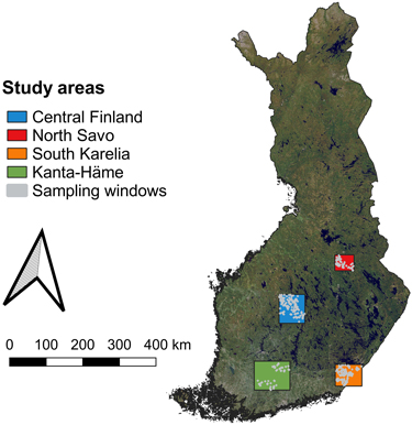
Fig. 1. Geographically dispersed study areas in Finland. The spatial distributions of the used sampling windows (i.e. field plots) within the study areas are also presented. The background raster contained data from the National Land Survey of Finland NLS orthophotos (accessed 4 April 2023 via open Web Map Tile Service, WMTS).
| Table 1. The four rectangular (in WGS 84 / UTM zone 35N, EPSG:32635) study areas named after the regions where they were located in Finland, and the Sentinel-2 MSI Level-2A products used in the study. The sun zenith angle corresponds approximately to the centre of the study area at the time of Sentinel-2 MSI image acquisition. Numbers in the size column are rounded to the closest kilometre. | |||||
| Name | Easting (m) | Size | Sun zenith angle | Sentinel-2 MSI Level-2A products | |
| min | max | ||||
| Northing (m) | |||||
| min | max | ||||
| Central Finland | 373960 | 444960 | 71 km × 79 km | 39.7° | S2A_MSIL2A_20190630T100031_N0212_R122_T35VLK_20190630T125130, S2A_MSIL2A_20190630T100031_N0212_R122_T35VMK_20190630T125130 |
| 6900320 | 6979320 | ||||
| North Savo | 526580 | 579340 | 53 km × 44 km | 40.6° | S2A_MSIL2A_20190614T094031_N0212_R036_T35VNL_20190614T111852 |
| 7043660 | 7087340 | ||||
| South Karelia | 527900 | 600900 | 73 km × 59 km | 38.1° | S2A_MSIL2A_20200615T093041_N0214_R136_T35VNH_20200615T120311 |
| 6728920 | 6787920 | ||||
| Kanta-Häme | 306000 | 403800 | 98 km × 79 km | 38.8° | S2A_MSIL2A_20190710T100031_N0213_R122_T35VLH_20190710T114201 |
| 6718240 | 6797040 | ||||
2.2 Forest data
2.2.1 Inventory field plots
The forest ground truth data of the study were provided by the Finnish Forest Centre, which collects forest inventory data by combining field plot measurements, airborne laser scanning data and aerial images. The aim of the field measurements is to cover the inventoried areas as well as possible in terms of variability of forests (different species, densities, sizes and site types). The Finnish Forest Centre distributes the plot level forest resource data under Creative Commons Attribution 4.0 International (CC BY 4.0) license. More information on the inventory process is given by Maltamo et al. (2011) and Holopainen et al. (2015).
We used the inventory field plots with a radius of 9 m as our forest ground truth data. The trees growing in the field plot are distributed into classes according to species and age. A single class, called a stratum, thus includes a homogeneous set of trees in terms of age, height and species. The typical number of strata per field plot was 1–3. The following variables, determined as a part of the forest inventory for each stratum, were used in the study: mean diameter at breast height (1.3 m, tree basal area weighted, unit: cm), mean height (tree basal area weighted, unit: m), basal area of the stratum (unit: m2 ha–1), stem volume (over bark, unit: m3 ha–1), stem count (unit: ha–1) and tree species. Other structural variables required for forest reflectance modelling were predicted using allometric relationships (Section 2.5.2 “Forest structural information in FRT”) for boreal forests.
2.2.2 Selection of field plots
We only used field plots with fertility classes 2 (herb-rich, OMT), 3 (mesic, MT), 4 (sub-xeric, VT) and 5 (xeric, CT) based on Cajander’s (1926) theory of forest types due to the availability of forest floor reflectance data in the utilised spectral database of understorey vegetation measurements (Section 2.4.1 “Understorey vegetation spectra”). Furthermore, we limited the data to the year corresponding with the acquisition of the Sentinel-2 Multispectral Instrument image (Section 2.3 “Remote sensing data”) used for each study area (Table 1) to avoid temporal difference between remote sensing and forest data.
We excluded plots with only small trees by setting thresholds for plot level mean diameter and stem volume, computed from the stratum-specific data as basal area weighted mean and total sum, respectively. For mean diameter we used a minimum of 8 cm, which is a threshold for Finnish seedling stands (Äijälä et al. 2019). For stem volume, we used a minimum of 10 m3 ha–1, the smallest mean volume of growing stock on Finnish forest land reported in the Multi-source National Forest Inventory 2011 (Tomppo et al. 2014). In addition, we excluded plots with unrealistically long plot level crown length exceeding 95% of the plot level mean tree height. The plot level values were computed from stratum-specific data as basal area weighted mean. It is worth noting, however, that in nature crown lengths of spruce may be relatively long compared with tree height, especially in sparse stands.
2.3 Remote sensing data
We used the optical remote sensing data by Sentinel-2 Multispectral Instrument (MSI) from the peak growing season, 14 June 2019, 15 June 2020, 30 June 2019 and 10 July 2019 for North Savo, South Karelia, Central Finland and Kanta-Häme, respectively. The images were downloaded from Copernicus Open Access Hub as Level-2A products that provide directly bottom of atmosphere reflectances (scaled between 1 and 10 000). The images had been acquired between 9:30 and 10:01 AM (UTC), and the sun zenith angle varied in the study areas between 38.1° and 40.6° (Table 1). We used Sentinel-2 MSI bands in the visible and near infrared spectral regions: B2, B3, B4, B5, B6, B7, B8 and B8A with central wavelengths of 490, 560, 665, 705, 740, 783, 842 and 865 nm, respectively. The Sentinel-2 MSI bands with 60 m spatial resolution, i.e. B1 (443 nm) and B9 (940 nm), were not used. In addition, we did not use the bands in the shortwave infrared (SWIR) spectral region, i.e. B11 (1610 nm) and B12 (2190 nm), as the hyperspectral measurements of stem bark did not include the SWIR region (Section 2.4 “Hyperspectral in situ data”).
We created 40 m × 40 m sampling windows around the field plots corresponding to 4 × 4 pixels of the Sentinel-2 MSI bands with the highest spatial resolution. We used the forest stand geometries provided by the Finnish Forest Centre to exclude windows that were not fully inside forested area, i.e. we excluded the plots on forest edge and close to roads or agricultural fields. In addition, we did not use the plots that were close to small clouds in the Sentinel-2 MSI image of Kanta-Häme study area. The images of the other study areas were cloudless. Furthermore, we filtered out windows where the standard deviation of the surface reflectance of the NIR band (B8) was above 0.025 to exclude the windows that were overly heterogeneous, e.g. located on stand boundaries or might have suffered from illumination distortions due to slopes and hills. Finally, we excluded the windows that had their NDVI values in the lowest five percent to remove areas with low vegetation, e.g. logged areas. In total, 927 sampling windows were retained (Table 2). For each window, we calculated the zonal mean reflectances from the Sentinel-2 MSI data (Fig. 2).
| Table 2. Forest characteristics of the field plots used for each study area. Plot level mean values for diameter, tree height, basal area, stem volume and stem count are given. The second given value in the brackets is the interquartile range, which is defined as the difference between the 75th and 25th percentiles of the data. Forest reflectances were simulated using forest reflectance and transmittance model FRT for these field plots. | ||||||
| Study area | Number of sampling windows | Mean diameter (cm) | Mean tree height (m) | Mean basal area (m2 ha–1) | Mean stem volume (m3 ha–1) | Mean stem count (ha–1) |
| Central Finland | 430 | 20.4 (7.0) | 17.7 (5.7) | 22.7 (10.7) | 204 (121) | 1028 (550) |
| North Savo | 113 | 13.9 (5.1) | 12.1 (4.0) | 16.5 (8.5) | 105 (71) | 1650 (1022) |
| South Karelia | 257 | 17.3 (8.0) | 15.8 (7.2) | 23.9 (12.5) | 200 (154) | 1542 (903) |
| Kanta-Häme | 127 | 16.7 (8.6) | 15.2 (7.0) | 23.0 (9.7) | 184 (117) | 1664 (1042) |
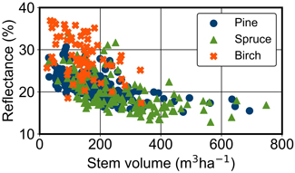
Fig. 2. Stem volumes (m3 ha–1) and Sentinel-2 MSI reflectances of near infrared band (B8, λ = 842 nm) from the Central Finland study area. All sampling windows are presented (N = 430) and the dominant tree species are visualised with the symbols.
2.4 Hyperspectral in situ data
2.4.1 Understorey vegetation spectra
We used hyperspectral measurements of understorey vegetation hemispherical-conical reflectance factors (HCRF) from different types of boreal forest stands measured by Forsström et al. (2021a,b). The measurements had been carried out in 36 study stands differing in site fertility, species composition and structure in Hyytiälä, Finland between mid-June and mid-July in 2018 and 2019. The dataset of the measurements included forest floor reflectances (350–2300 nm) from 15 different sampling positions in each stand. Basal area, tree height, species composition and forest site type (OMT, MT, VT or CT) based on Cajander’s (1926) theory of forest types were provided for the 36 stands with the spectral data. We computed the median reflectance factor for each wavelength for each stand.
In forest reflectance simulations, we selected the most suitable forest floor spectrum (from the 36 available) for each sampling window (i.e. field plot) using a simple support-vector machine (SVM) classification trained on the stand characteristics provided with the spectral data. The SVM classification was implemented using default parameter values with scikit-learn that is a well-known machine learning library for Python programming language (Pedregosa et al. 2011). We trained a separate SVM classifier for each site fertility type (i.e. OMT, MT, VT and CT). The training data for the classifiers included species composition (percentages for pine, spruce, birch and other species), basal area and tree height, and the target values were the corresponding study stand numbers. When predicting the stand number for the most suitable spectrum, the trained SVM classifier was selected based on the site fertility of the field plot, after which the input features required for the prediction were gathered from the plot data. Further, to study the relevance of forest floor spectrum to the simulation accuracy of forest reflectance, we also simulated the forest reflectance with a spectrum based on the site fertility but otherwise chosen randomly.
2.4.2 Foliage spectra
For foliage spectra, we used the data measured by Hovi et al. (2022a,b). The measurements were carried out in Hyytiälä, Finland (1–11 July 2019), Bílý Kříž, the Czech Republic (19–21 September 2019), and Järvselja, Estonia (2–17 July 2020). A total of 27 Scots pine, Norway spruce, silver birch (Betula pendula Roth), European aspen (Populus tremula L.) and black alder (Alnus glutinosa (L.) Gaertn.) trees were sampled. The hyperspectral data included reflectance and transmittance factors (350–2500 nm) for the two sides of the leaves (adaxial and abaxial). Two canopy positions (bottom-of-canopy and top-of-canopy) had been sampled for each tree with three samples for each position. For conifers, current-year and one-year-old needles had been sampled separately, doubling the number of samples. Together with the leaf spectrum and species, tree height and diameter at breast height (DBH) were recorded.
For conifers, we averaged reflectance and transmittance spectra from both sides of the needles (adaxial and abaxial), current-year and one-year-old needles and both canopy positions. For broadleaved species (i.e. birch), we used two scenarios (Fig. 3): (1) we averaged the spectral data from the upper (adaxial) side of the leaves, assuming that it dominates the reflectance spectrum, and both canopy positions, and (2) we averaged the spectral data from both sides of the leaves and both canopy positions. The former scenario was used primarily (Section 2.6 “Analyses”). The foliage spectrum was selected separately for each simulated tree class based on tree species and the smallest sum of relative errors for DBH and tree height.
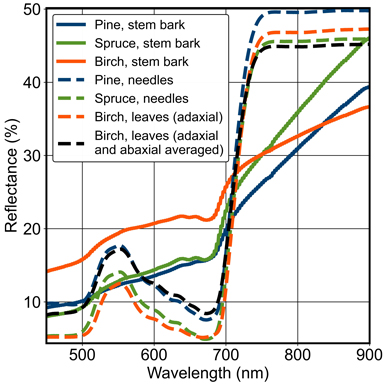
Fig. 3. Stem bark reflectance spectra of pine, spruce and birch used in the study. Examples of foliage reflectance spectra of pine, spruce and birch are also presented from Hyytiälä, Finland. For birch leaves, two different spectra are presented: the upper (adaxial) side and the average of the upper and bottom (abaxial) sides. For the conifers, the two sides were averaged.
2.4.3 Stem bark spectra
We used hyperspectral measurements by Juola et al. (2022a,b) for tree trunks and branches. The measurements had been carried out between May and August in 2020 near Helsinki, Finland and Järvselja, Estonia. The dataset included hemispherical-directional reflectance factors (HDRFs, 400–1000 nm) for ten common boreal and temperate tree species, including the same species as for the foliage spectra. The reflectance factors provided in the dataset were averaged from 20 samples. In forest reflectance simulations, we selected the spectral data based on tree species, i.e. pine, spruce or birch (Fig. 3).
2.5 Forest reflectance simulations
2.5.1 Forest radiative transfer model
We used the forest reflectance and transmittance model FRT (Kuusk and Nilson 2000) to simulate the forest reflectance spectra. The model describes forests as a group of geometrical trees from one or more tree classes that differ in species (i.e. optical properties of tree elements), age and size. FRT is a hybrid geometric-optical forest reflectance model computing the spectral radiance of a forest stand as a sum of the single scattering radiance of direct solar flux and the radiance of diffuse fluxes that originate from multiple scattering and scattered diffuse sky flux (Kuusk et al. 2010). The geometric-optical submodel used for first-order scattering assumes a random distribution for the branches and foliage of the tree crowns, and a spherical leaf angle distribution for the leaves and needles. The two-stream radiative transfer submodel for modelling the higher-order scattering assumes a random distribution of foliage elements. The grouping of conifer needles into shoots is accounted for in both submodels by using the shoot as the basic scattering unit. The shoot scattering albedo was computed using the recollision probability concept (Rautiainen et al. 2012) while retaining the measured spectral reflectance to transmittance ratio of the needles. Due to different parametrisations of the canopy structure between the submodels, the two-stream submodel requires a correction to fulfil the law of energy conservation in order to be coherent with the geometric-optical part (Mõttus et al. 2007). We normalised the model to conserve energy using leaf properties at 550 nm.
FRT can model stand level reflectance and transmittance factors of a forest at specific wavelengths for a given solar angle and direction. The hyperspectral data described above were used as the spectral properties of forest elements (forest floor, bark, leaves and needles). We used FRT to simulate HDRFs in the wavelength range 450–950 nm and applied the Sentinel-2 spectral response functions to obtain the simulated reflectances for the Sentinel-2 MSI bands B2–B8A (Fig. 4).
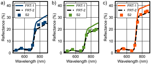
Fig. 4. Examples of forest reflectance simulations by the forest reflectance and transmittance model FRT (FRT-1 and FRT-2) compared with Sentinel-2 (S2) MSI data for pure a) pine, b) spruce and c) birch field plots in Kanta-Häme study area in Finland. Baseline values from Table 3 and adjusted values from Fig. 5 were used as FRT input parameters for FRT-1 and FRT-2, respectively.
2.5.2 Forest structural information in FRT
Mean tree height (m), mean diameter (cm) and stem count (ha–1) were directly input to FRT from the field plot data. Species-specific allometric regression models from literature were used for the rest of the variables using mean tree height and diameter as independent variables. Crown radius and length (m) of pine and spruce were predicted using linear regressions developed by Rautiainen et al. (2008) for Finland. For broadleaved species (i.e. birch), crown radius was predicted using a model by Jakobsons (1970) for northern Sweden and crown length using a model by Nilson et al. (1999) for Estonia. Dry leaf weight (kg tree–1) was predicted using models developed by Repola (2008, 2009), with the exception of birches with mean diameter < 11 cm, where we used Johansson’s (1999) model as suggested by Majasalmi et al. (2013): the Repola model yields unrealistic values for small birches.
In FRT, the spatial structure of the forest is quantified by the tree distribution parameter (TDP), which is connected to the Fisher’s Grouping Index (GI), the relative variance of the number of trees on a plot with an area that equals to the vertical projection area of a tree, as TDP = –ln(GI) / (1–GI) (Nilson 1999). GI, and thus TDP, indicates whether the tree distribution is regular, random or clumped. GI < 1 corresponds to a regular distribution, typical for a managed boreal forest. A completely random spatial pattern generated by a Poisson process produces GI = 1, and in a clumped forest GI > 1. In nature, TDP can vary with site type, tree species and especially management background, and it should not be identical in every forest. However, there exists no reliable data based on which an optimal TDP could be selected for a specific forest. Consequently, we used a single estimate for each tree species and for each study area (Supplementary file S1).
2.5.3 Observation conditions
We used the same atmospheric data for each study area: continental aerosol model with an aerosol optical depth of 0.06 corresponding to a summer day with clear skies in Finland and representative of the acquisition dates of the Sentinel-2 MSI data (Table 1). Viewing and illumination geometry of the modelled scene corresponded to the actual Sentinel-2 MSI data.
2.6 Analyses
First, we defined baseline values for the FRT input parameters (Table 3) based on previous published research. We then started to adjust the input parameters to improve the agreement between the forest reflectance simulations and measured reflectance data by Sentinel-2 MSI. The investigations of the influence of FRT input modifications were carried out for the Kanta-Häme study area (127 sampling windows).
| Table 3. Forest reflectance and transmittance model FRT input parameters and their baseline values. The origin of the value is described in the source column. | ||
| Parameter | Baseline values | Source |
| Specific leaf weight (g m–2), SLW | Pine 158, Spruce 200, Birch 57 | As used by Hovi et al. (2016) |
| Branch area to leaf area ratio, BAILAI | Pine 0.18, Spruce 0.18, Birch 0.15 | As used by Rautiainen and Lukeš (2015) and Hovi et al. (2016) |
| Shoot shading coefficient, SSC | Pine 0.59, Spruce 0.64, Birch 1.00 | As used by Rautiainen and Lukeš (2015) and Hovi et al. (2016) |
| Shoot length (m), SHL | Pine 0.10, Spruce 0.05, Birch 0.40 | As used by Hovi et al. (2016) |
| Tree distribution parameter, TDP | 1.2 for all species | As used by Hovi et al. (2016) |
| Tree height (m) | Forest data | Finnish Forest Centre |
| Trunk diameter (cm) | Forest data | Finnish Forest Centre |
| Density (m–2) | Forest data | Finnish Forest Centre |
| Tree species | Forest data | Finnish Forest Centre |
| Dry leaf weight (kg tree–1), DLW | Allometric regression models from literature and forest data | Repola (2008, 2009) and Johansson (1999) |
| Crown radius (m) | Allometric regression models from literature and forest data | Rautiainen et al. (2008) and Jakobsons (1970) |
| Crown length (m) | Allometric regression models from literature and forest data | Rautiainen et al. (2008) and Nilson et al. (1999) |
We adjusted the values of several uncertain input parameters for which we did not have quality or routinely measured empirical data available, and we knew the theoretical definition but lacked the comprehensive understanding or details. From the FRT input parameters (Table 3), we regarded tree distribution parameter (TDP), shoot length (SHL), branch area to leaf area ratio (BAILAI), shoot shading coefficient (SSC), specific leaf weight (SLW) and the crown dimensions (i.e. crown radius and length) as uncertain parameters. The other FRT inputs, apart from dry leaf weight (DLW), were directly read from the forest data and represented state-of-the-art structural properties. The allometric models used for DLW were also the best available.
We studied the influence of the input parameter adjustment to the estimation accuracy across all Sentinel-2 MSI bands in terms of Pearson correlation coefficient (r), relative root-mean-square error (coefficient of variation, rRMSE, Eq. 2) and normalised mean bias (NMB, Eq. 3),


where Mi is the modelled forest reflectance, Oi the corresponding observed Sentinel-2 MSI reflectance, Ō the mean of the observed reflectances and N the number of sampling windows per study area (Table 2). RMSE is a widely used error metric for numerical predictions. It aggregates the magnitudes of the errors in predictions into a single measure of accuracy. Mean bias is primarily used to estimate the average bias in the model. Consequently, it serves as a quantification of the systematic error of the model. As one of our study objectives was to decrease the possible systematic prediction error of forest reflectance in different spectral regions, we concentrated on obtaining a NMB value close to zero for each Sentinel-2 MSI band while keeping the rRMSE values as low as possible and r as high as possible. Compromises were made as we searched for the balance across all Sentinel-2 MSI bands.
We started the parameter adjustment with TDP, as it was optimised and estimated separately. We estimated a new value for TDP by minimising the difference between measured and estimated canopy transmittance. From the calculations (detailed in Suppl. file S1) we obtained a single value that was used for each tree species and tree class in the FRT simulations. However, it should be noted that the FRT model adjusted the used TDP of a tree class, if the canopy cover computed by the model would have been greater than the crown cover, which is not possible in reality. In such cases, a new GI was calculated for the tree class by subtracting its crown cover from one (Nilson and Kuusk 2004). After which, the model calculated the adjusted TDP from the new GI.
We then adjusted the remaining uncertain input parameters one after another, based on existing understanding of their effect on forest spectral reflectance and the current uncertainty in their values. We thus began with SHL followed by BAILAI, SSC, SLW, crown radius and length. The order was influenced by the fact that we did not want to adjust SLW in the beginning, since modifying it would have changed the leaf area index computed and used by FRT. Further, the crown dimensions were adjusted last, as the used regression models were the best available, while we also knew that they were not perfect. The order for SHL, BAILAI and SSC was arbitrary, and other order could have also been used, which might have produced slightly different final set of adjusted parameters. The aforementioned parameters had species-specific values for pine, spruce and birch, which were increased and decreased individually or simultaneously. Different combinations were tested (Suppl. file S2), and the effects of the modifications were analysed in the Sentinel-2 MSI bands. With SHL, we studied nine different combinations in which the modifications to the species-specific values were between 2 and 30 cm compared with the baseline values. With BAILAI, we mainly increased the species-specific values, as we noticed that decreasing had undesirable effect. Different BAILAI values were tested between 0.07 and 0.35, and in total 17 combinations were studied. With SSC, we investigated in total 11 different combinations in which species-specific values were between 0.4 and 1.2; values for conifers did not exceed 0.9. With SLW, we carried out an extensive investigation including 14 different combinations of species-specific values. For pine, the values were between 115 and 200 g m–2, for spruce 152 and 210 g m–2 and for birch 20 and 76 g m–2. With crown dimensions, the species-specific values were modified by a certain percentage. Modifications to crown radii were between –15% and +10%, and to crown lengths between –25% and +5%. With crown radius and length, we studied in total 15 and 7 different combinations, respectively.
In addition to the adjustment of the uncertain parameters, we analysed the influence of foliage and forest floor spectra to the estimation accuracy. For the foliage spectra of broadleaved trees (i.e. birches), we used primarily the spectral data only from the upper side of the leaves, as we assumed that in reflectance signal formation the reflectance from the upper side dominates. However, we also investigated the estimation accuracy when averaging the spectral data from both sides of the leaves, similarly as we did with conifers. Furthermore, we tested to select the forest floor spectra randomly, in place of the SVM classification: the only common factor between the used spectrum and a sampling window was the site fertility type.
After adjusting the FRT input parameters (Fig. 5), the species-specific modelling performance of FRT was explored using scatterplots of forest reflectance estimations for pure (i.e. single species) pine, spruce and birch field plots.
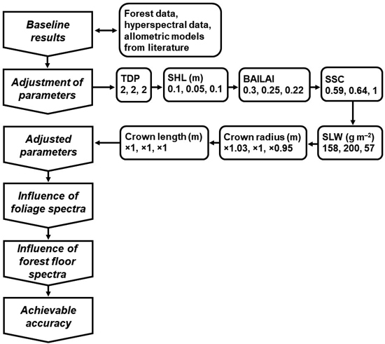
Fig. 5. A flowchart of the analyses including the adjusted FRT input parameter values. The three numbers below the names of the input parameters correspond to the species-specific values for pine, spruce and birch, respectively. For crown radius and length, the numbers are the coefficients used to modify the allometry-based values. See Table 3 for the parameter names and abbreviations.
3 Results
3.1 Parameter adjustments
The estimation of the new TDP value (detailed in Suppl. file S1) led to TDP = 2 (GI = 0.203) for Finnish boreal forest. Based on the other input parameter adjustments, we decided on changing SHL only for birch. The new value was 0.10 (Fig. 5). The species-specific values of BAILAI were also changed. The new values were 0.30 for pine, 0.25 for spruce and 0.22 for birch. With SSC and SLW, we decided on using the baseline values because we achieved only minor improvements. With the crown dimensions, we ended up changing values only for crown radii of pine and birch. We increased pine crown radius by 3% and decreased birch crown radius by 5%. We did not gain benefit from adjusting the crown length of any species.
3.2 Estimation accuracy with the new hyperspectral in situ data
With the baseline input parameter values (Table 3), rRMSE values were between 16% and 39% for each study area (Table 4). In general, forest reflectance simulations in the near infrared (NIR) spectral region (Sentinel-2 MSI bands B6–B8A) tended to be less accurate. In NIR, rRMSE values were on average ca. 36%, 29%, 27% and 25% and in the visible (VIS) spectral region (Sentinel-2 MSI bands B2–B5) ca. 27%, 22%, 25% and 23% for Central Finland, North Savo, South Karelia and Kanta-Häme, respectively. Biases (i.e. NMBs) differed between the Sentinel-2 MSI bands more than the rRMSE values. The variation of biases was notable especially in VIS, whereas in NIR biases were of a similar magnitude for each study area (Table 4).
| Table 4. Estimation accuracy (relative root-mean-square error, rRMSE), correlation (Pearson correlation coefficient, r) and bias (normalised mean bias, NMB) for the simulated forest reflectance in eight Sentinel-2 MSI bands (B2–B8A) with the baseline input parameter values (Table 3). | |||||||||
| Study area | B2 | B3 | B4 | B5 | B6 | B7 | B8 | B8A | |
| Central Finland | r | 0.62 | 0.67 | 0.49 | 0.73 | 0.80 | 0.78 | 0.78 | 0.77 |
| rRMSE (%) | 38.8 | 24.5 | 28.8 | 15.9 | 34.0 | 36.2 | 34.8 | 37.4 | |
| NMB (%) | 31.4 | 16.4 | 7.2 | 5.0 | 29.6 | 31.9 | 30.9 | 33.7 | |
| North Savo | r | 0.58 | 0.50 | 0.61 | 0.61 | 0.77 | 0.76 | 0.75 | 0.74 |
| rRMSE (%) | 21.5 | 17.4 | 31.2 | 18.8 | 25.7 | 29.3 | 30.9 | 30.8 | |
| NMB (%) | 5.4 | –0.1 | –1.9 | –6.8 | 21.8 | 25.6 | 27.7 | 27.7 | |
| South Karelia | r | 0.13 | 0.23 | 0.26 | 0.56 | 0.77 | 0.75 | 0.75 | 0.74 |
| rRMSE (%) | 26.9 | 22.8 | 29.1 | 19.3 | 24.0 | 26.7 | 29.2 | 27.5 | |
| NMB (%) | –15.7 | –9.4 | –15.0 | –11.5 | 17.4 | 20.8 | 24.3 | 22.7 | |
| Kanta-Häme | r | 0.51 | 0.51 | 0.44 | 0.69 | 0.82 | 0.79 | 0.80 | 0.79 |
| rRMSE (%) | 21.1 | 26.1 | 26.4 | 19.1 | 26.4 | 24.5 | 23.4 | 25.1 | |
| NMB (%) | 5.8 | 15.6 | 12.4 | 11.1 | 21.5 | 19.4 | 18.8 | 20.7 | |
3.3 Effect of the adjusted values of the uncertain parameters
The increase in TDP, meaning a more regular and closed canopy, decreased biases on average by ca. 8 percentage points (pp) in VIS and 7 pp in NIR (Fig. 6). The rRMSE values decreased by about 3 pp in VIS and 5 pp in NIR. Correlations improved only a little in NIR (r increased by 0.01). In VIS, correlation coefficients decreased by 0.02–0.04. The change of TDP influenced the modelling performance similarly also in the other study areas.
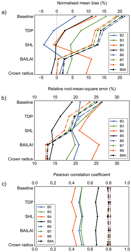
Fig. 6. The change of performance metrics for the baseline scenario and after adjusting the tree distribution parameter (TDP), shoot length (SHL), branch area to leaf area ratio (BAILAI) and crown radius in Kanta-Häme study area in Finland. The presented metrics for eight Sentinel-2 MSI bands (visible region B2–B5 and near infrared region B6–B8A) are a) normalised mean bias, b) relative root-mean-square error and c) Pearson correlation coefficient.
Adjusting the SHL of birch decreased biases by ca. 3 and 1 pp and rRMSE values by ca. 2 and 1 pp in VIS and NIR, respectively. Correlations improved in VIS (r increased by 0.02–0.05). In NIR, correlation coefficients decreased by 0.01. The modified value for birch influenced the modelling performance similarly also in the Central Finland study area. In the remaining two study areas, only minor differences occurred for bands B4 and B5.
Modifying the BAILAI values induced major changes in accuracy in NIR, as biases decreased by ca. 11 pp and rRMSE values by ca. 5 pp. Correlation coefficients increased by 0.01 or remained the same. In VIS, the effects varied. Depending on the band, accuracies and biases were slightly poorer (< 2 pp) or they weakened several percentage points, e.g. for the red band (B4) the bias weakened from –1.0% to 11.0% and the rRMSE value increased from 20.9% to 25.7%. Nevertheless, the modifications made to BAILAI decreased the overall magnitude of biases and rRMSE values considerably (Fig. 6). The modelling performance was similar in all study areas.
The modifications to the allometric crown radii of pine and birch decreased biases in VIS and NIR on average by 1 pp. In NIR, absolute values of biases reached < 2% for each band. We succeeded to retain or improve accuracy for each band. The rRMSE values decreased by less than 1 pp in NIR and by 1–2 pp in VIS. Correlation coefficients increased in VIS by 0.01–0.04 and decreased by 0.01 or remained the same in NIR. The modifications affected similarly the modelling performance also in the other study areas.
3.4 Influence of spectral properties of leaves and forest floor
The reflectance of the upper (adaxial) side of birch leaves was lower than that of the mean of both sides in the visible part of the spectrum (Fig. 3). Using the mean of adaxial and abaxial reflectances as the leaf reflectance in FRT increased greatly (on average by 13 pp) biases in VIS and weakened correlations: rRMSE values increased by 17 pp and 15 pp, respectively, for green (B3) and red band (data not shown). The biases were too large to be corrected with adjustments in other uncertain parameters. In NIR, the effects on biases and rRMSE values were minor and correlations did not change.
The method for selecting the forest floor spectrum did not affect the simulation accuracy substantially. For the method that chose the spectrum randomly, rRMSE values and biases decreased ca. 1 pp in NIR; in the visible part of the spectrum, biases were on average the same and rRMSE values increased on average only by 0.3 pp. Hence, the differences were negligible. The correlation coefficients for the random method were 0.01–0.04 larger in both spectral regions. Overall, random (site fertility-based) forest floor spectra produced slightly better accuracy than the selection using SVM in NIR and vice versa in VIS. Canopy cover values computed by FRT for the simulated forests ranged between 0.579 and 0.998 in the Kanta-Häme study area (Fig. 7).
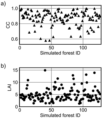
Fig. 7. The values of a) canopy cover (CC) and b) leaf area index (LAI) computed by the forest reflectance and transmittance model FRT for the simulated forests (N = 127) in Kanta-Häme study area in Finland.
3.5 Quantifying the achievable accuracy of FRT
With the adjusted set of input parameter values (Fig. 5), rRMSE values were between 13% and 33% for all study areas (Table 5). Contrary to the baseline results, forest reflectance estimations with the adjusted parameter values were more accurate in NIR: rRMSE values were on average ca. 23%, 23%, 27% and 19% in VIS, whereas in NIR, the adjusted set of inputs produced average rRMSE values of ca. 19%, 16%, 15% and 13% for Central Finland, North Savo, South Karelia and Kanta-Häme, respectively.
| Table 5. Estimation accuracy (relative root-mean-square error, rRMSE), correlation (Pearson correlation coefficient, r) and bias (normalised mean bias, NMB) for the simulated forest reflectance in eight Sentinel-2 MSI bands (B2–B8A) with the adjusted set of input parameter values (Fig. 5). | |||||||||
| Study area | B2 | B3 | B4 | B5 | B6 | B7 | B8 | B8A | |
| Central Finland | r | 0.64 | 0.67 | 0.50 | 0.68 | 0.76 | 0.74 | 0.73 | 0.71 |
| rRMSE (%) | 33.0 | 16.2 | 25.9 | 16.0 | 17.8 | 19.3 | 19.1 | 20.7 | |
| NMB (%) | 25.7 | 4.1 | 4.3 | –7.0 | 8.1 | 9.9 | 9.8 | 12.6 | |
| North Savo | r | 0.58 | 0.49 | 0.60 | 0.57 | 0.74 | 0.73 | 0.71 | 0.70 |
| rRMSE (%) | 19.3 | 19.2 | 29.1 | 24.2 | 13.8 | 15.5 | 16.8 | 16.7 | |
| NMB (%) | 0.3 | –10.2 | –6.5 | –17.4 | 3.3 | 6.5 | 8.9 | 9.3 | |
| South Karelia | r | 0.19 | 0.27 | 0.30 | 0.58 | 0.77 | 0.75 | 0.74 | 0.74 |
| rRMSE (%) | 27.8 | 25.9 | 28.7 | 25.4 | 14.4 | 15.2 | 15.6 | 15.0 | |
| NMB (%) | –19.4 | –19.1 | –17.1 | –21.8 | –1.8 | 1.0 | 4.4 | 3.5 | |
| Kanta-Häme | r | 0.51 | 0.53 | 0.45 | 0.67 | 0.82 | 0.80 | 0.81 | 0.79 |
| rRMSE (%) | 19.6 | 17.8 | 24.0 | 13.7 | 12.8 | 13.2 | 12.8 | 13.2 | |
| NMB (%) | 1.0 | 3.3 | 9.4 | –1.7 | 1.9 | 0.0 | –0.0 | 1.9 | |
In VIS, the average rRMSE values with the adjusted input parameters were of a similar magnitude compared with the baseline results. In NIR, the average rRMSE values decreased considerably, i.e. by 17 pp, 13 pp, 12 pp and 12 pp for Central Finland, North Savo, South Karelia and Kanta-Häme, respectively. Scatterplots of the forest reflectance simulations by FRT compared with Sentinel-2 MSI data (bands B2–B8A) for the Kanta-Häme study area are in Suppl. file S3.
3.6 Quantified bias for different tree species
The species-specific biases were in general the lowest for pine (Fig. 8). In VIS, the reflectance of pine and spruce forests were mainly underestimated and that of birch forests overestimated. The average absolute biases for pine, spruce and birch were approximately 7%, 19% and 18%, respectively. In NIR, FRT produced only small overestimations for each species: the average absolute biases for pine, spruce and birch forest reflectance were 4%, 3% and 4%, respectively.
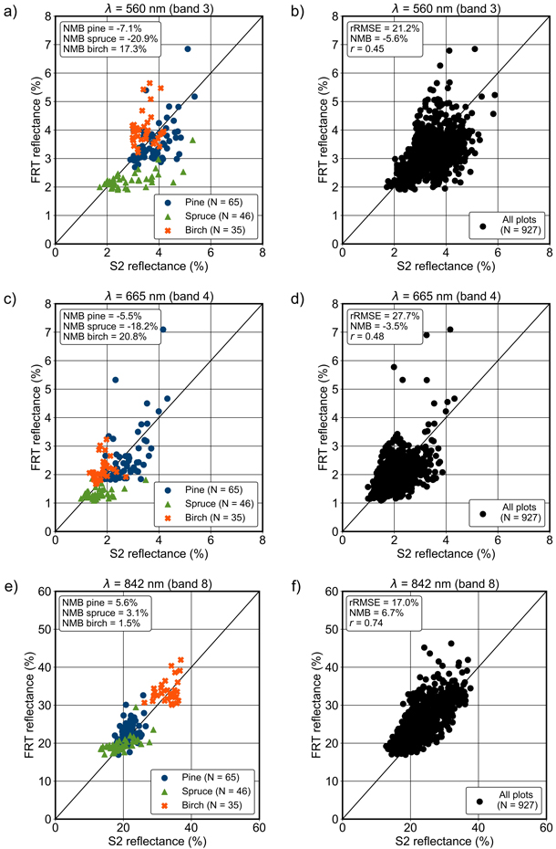
Fig. 8. FRT-simulated reflectances using the adjusted set of input parameter values in a, b) green, c, d) red and e, f) near infrared bands (for wavelengths 560, 665 and 842 nm, respectively) compared with Sentinel-2 (S2) MSI data. All pure pine, spruce and birch field plots in each study area (a, c and e), and all the used field plots combined (b, d and f, N = 927). The normalised mean bias (NMB), relative root-mean-square error (rRMSE) and Pearson correlation coefficient (r) are given in the subfigures.
The simulated reflectance of spruce forests varied the least in each band (Suppl. file S4), even though the variation of spruce forests was typically the largest in the measured Sentinel-2 MSI data. For example, in the green band the standard deviation of the simulated reflectance was 0.007 for pine, 0.0033 for spruce and 0.0058 for birch, whereas in the Sentinel-2 MSI data it was 0.0058, 0.0083 and 0.0038, respectively. In NIR band, the standard deviation of the simulated forest reflectances was 0.0282 for pine, 0.0193 for spruce and 0.0277 for birch, whereas in the Sentinel-2 MSI data it was 0.021, 0.0375 and 0.0267, respectively. Again, the variation in the simulated reflectance of spruce forests was overly small, while the variation in the reflectance of birch forests was modelled most accurately in NIR.
4 Discussion
4.1 Influence of structural FRT input parameter values
The state-of-the-art spectral and structural forest information allowed us to identify two input parameters influencing the most the modelling performance: tree distribution parameter (TDP, Fig. 6) and the branch area to leaf area ratio (BAILAI). In the FRT model, TDP quantifies the spatial structure of the modelled forest, and is uniquely connected to the Fisher’s Grouping Index GI (Suppl. file S1). TDP is not explicitly dependent on tree species but on the horizontal structure of the forest and scale. As we increased the value of TDP from 1.2 to 2, GI decreased from 0.686 to 0.203, indicating a more regular spatial structure of the forest. The positive effect of increasing the regularity of the spatial structure was expected due to the management practices in Finland (Kuusk et al. 2010; Rautiainen and Lukeš 2015). The large effect of the horizontal structure of a forest on its spectral reflectance gives hope to the possibility of separating managed production forests with regular structure (large TDP) from natural unmanaged forests, which tend to have a grouped structure (small TDP) and may also have a high forest diversity due to the combination of the less regular horizontal structure and a great variation in tree age, size and species composition. The task will not be trivial, as the changes in the spatial structure affect all spectral regions simultaneously and quite similarly, but our results merit further research on the topic.
The importance of woody materials in forest reflectance modelling has been emphasised already in previous published research (Malenovský et al. 2008; Verrelst et al. 2010; Kuusinen et al. 2021; Hovi et al. 2022c). Our findings supported this, as the influence of BAILAI, which is essentially a weight to average branch and needle spectra within FRT, was found to be considerable (Fig. 6), especially in NIR, and in the blue and red wavelength regions of VIS corresponding to the absorption peaks of chlorophyll. The adjusted species-specific BAILAI values (Fig. 5) for pine, spruce and birch were 67%, 39% and 47%, respectively, above the baseline. In VIS, the reflectance of non-photosynthetic vegetation, e.g. stem and branch bark, is characterised by a gradual increase with wavelength. The reflectance of stem bark is clearly higher than that of needles and leaves in red and blue. In green, this holds only for birch (Fig. 3). Due to this, the underestimations of FRT-simulated forest reflectance in the blue and red bands changed to overestimations with the increase in BAILAI (Fig. 6). In NIR, however, adding woody material decreases forest reflectance and thus reduced overestimations by FRT, since the reflectance of stem bark is lower than that of foliage after 700 nm for all used tree species (Fig. 3). Similar influences of branch spectrum on forest reflectance have been reported by Malenovský et al. (2008) and Hovi et al. (2022c).
The adjusted BAILAI values (Fig. 5) described the ratio between branch area and leaf area (BAI / LAI), whereas recent studies by Kuusinen et al. (2021) and Hovi et al. (2022c) used the ratio of woody elements to total plant area, PAI = LAI + BAI. In this study, the used BAI / PAI values were 0.23 for pine, 0.20 for spruce and 0.18 for birch. From the aforementioned studies, the former obtained average woody element contribution of 0.140–0.186 for pine, 0.090–0.095 for spruce and 0.116–0.196 for birch, depending on the used model, and the latter obtained 0.22 for pine, 0.21 for spruce and 0.12 for a mixture of broadleaved species. Some of these values were of similar magnitude to the ones recommended in this study. Due to the large sensitivity of forest reflectance on the amount of branch area, these values would lead to considerably different predictions of forest reflectance.
Based on the analysis of parameter adjustment, SHL values smaller than the baseline (Table 3) decreased biases, although the parameter should have an impact close to the hotspot. In NIR, we found no physically meaningful lower limit. In VIS, simulations ceased to improve after a threshold of using SHL = 0.10 m for pine and birch and SHL = 0.05 m for spruce. Using even smaller values would contradict the physical meaning of the parameter.
The effect of changing the crown radii of pine and birch was larger in VIS than in NIR, but its overall effect was small. This corresponds to the influence of forest floor reflectance: in boreal forests and at viewing angles close to nadir, the contribution of forest floor is above 40% and below 30% in VIS and NIR, respectively (Rautiainen and Lukeš 2015). However, it is worth noting that the used allometric regression models for the crown dimensions are not perfect. The model used for the crown radius of birch, for instance, seemed to predict overly wide crowns, as we achieved better accuracy by decreasing the predicted value.
4.2 Assessing the effect of forest floor and leaf spectra
A random site fertility-specific forest floor spectrum worked equally well or even better than a spectrum selected by the SVM algorithm. This may indicate a large variation in forest floor spectra within a single site fertility type and the existing spectral database does not capture it. The unavailability of a representative forest floor spectral database is one of the main current limitations in boreal forest reflectance simulations, which will inevitably lead to inaccuracy in reflectance model inversion. Another plausible explanation is that the canopy cover was large for some of the simulated forests (Fig. 7), and therefore only a small part of the forest floor was visible and thus its influence was small.
The abaxial side of a birch leaf has a strong spectrally invariant reflectance component with abaxial reflectance factors more than two times higher than that of adaxial side in the visible part of the spectrum. The effect is less evident in NIR where leaf reflectance is much larger (Fig. 3). This causes a problem in choosing suitable spectrum for reflectance simulations and reflectance model inversion. While mostly adaxial side is sunlit and visible to the sensor – especially for nadir viewing and small solar zenith angles – the radiation regime and diffuse reflectance are affected by both leaf sides, especially in NIR where multiple scattering dominates (Kuusk et al. 2010). In practice, however, using the averaged leaf reflectance from the two sides led to systematically unrealistic forest reflectance factors in VIS, making the use of the adaxial leaf reflectance an obvious choice. As a consequence of multiple scattering, the contribution of abaxial reflectance is larger in NIR than in VIS, and thus ignoring it would lead to modelling errors in this spectral region. Fortunately, in NIR the two sides are spectrally nearly identical. While detailed 3D models allow setting the optical properties of all canopy elements individually, we are not aware of any analytical canopy reflectance model that would allow using separate leaf reflectance values for the adaxial and abaxial sides. Therefore, we suggest using only the upper side of the leaves for the foliage spectra of broadleaved species. It is also worth bearing in mind that if one uses leaf optical model in FRT simulations, adjustment of the SLW input parameter affects leaf spectra in FRT. When using measured spectra (as done in this study) adjustment of SLW only affects the leaf area index computed and used by FRT.
4.3 Achieved modelling accuracy
Our analyses for the Kanta-Häme study area suggested that we were able to quantify the currently achievable accuracy of FRT in the wavelength range 740–950 nm (i.e. after the red edge), where the dynamic range of vegetation reflectance is the greatest: we achieved biases close to zero across all simulated wavelengths and rRMSE values close to 13%. In addition, in the other study areas biases were mostly below 10% and rRMSE values varied between 14% and 21% (Table 5). In the visible part of the spectrum, biases and rRMSE values varied much more in and between the study areas: the performance metrics were relatively good for Kanta-Häme and Central Finland, but for North Savo and South Karelia, we obtained large underestimations (Table 5).
One of the reasons for the differences between the regions could have been the different acquisition dates (Table 1) of Sentinel-2 MSI images. For Kanta-Häme, we used an image from 10 July, for Central Finland from 30 June, and the images for North Savo and South Karelia were acquired even earlier, on 14 and 15 June, respectively. The reflectance of boreal forests varies within the growing season. The mean reflectance in VIS was clearly higher for North Savo and South Karelia compared with Kanta-Häme and Central Finland, acquired several weeks later. In NIR, the differences were smaller. It is reasonable to assume that the differences in the Sentinel-2 MSI images contributed to the variation in performance metrics of the VIS region between the study areas.
We noticed that FRT has difficulties to simulate the reflectance of spruce forests with good accuracy and precision, especially in VIS (Fig. 8). The variation in the simulated spruce forest reflectances was overly small, and the biases in VIS region (bands B2–B5) were large and negative (on average –19%). In addition, the biases of the simulated pine forest reflectances were negative for bands B3–B5 (on average –8%). One possible contributing factor to the underestimated reflectance of conifer forests in VIS could be the wax surface of the needles that induces a specular reflectance that may not have been simulated correctly. Especially with spruce, the estimations were poor with the smallest wavelengths (Suppl. file S4). According to Markiet et al. (2017), specular reflectance increases in VIS with decreasing wavelength, and it is mostly directed in backward directions. This would lead to a higher canopy reflectance compared with a situation where the scattering would be partly directed in the forward directions. Another potential contributing factor could be the systematic underestimation of backward scattering reported by Kuusk et al. (2014). They found that the simulation accuracy of FRT could be improved by using erectophile leaf angle distribution (LAD). Alternatively, a few broadleaved trees inside the sampling window not captured by the plot measurements could alter the reflectance of a spruce forest. It is likely that the nature of the cause can be understood better with hyperspectral remote sensing data, e.g. by trying to detect wax reflectance spectrum in the reflectance signal similarly to Markiet et al. (2017).
4.4 Future outlooks
The discussion above allows to determine further actions with models and measurements for further elimination of the biases in simulated forest reflectance. Reflectance cannot be emulated with absolute accuracy as the location and spectral properties of each single scattering element cannot be determined on a large scale. Simplifications and abstractions (e.g. a tree crown filled semi-randomly with foliage elements) have proven to be useful and efficient but require proper parametrisations. A key characteristic for forest reflectance modelling is the spatial tree distribution pattern. The Fisher’s Grouping Index (GI) used by FRT has a solid theoretical definition (Nilson 1999), but more research is needed to determine the most appropriate GI for different types of forests, its natural range and the possibility to retrieve its value from remote sensing data – either from spectral information or very-high-resolution imagery where individual tree crowns can be identified.
A clear improvement in the representation of a forest would be the inclusion of different reflectance factors for adaxial and abaxial sides of foliage as this information is available from measurements and considering for the angular distribution of the scattering surfaces. Kuusk et al. (2014) studied the effect of LAD in FRT simulations in Estonian hemiboreal forests and found that the use of erectophile LAD instead of spherical helped to improve the simulated gap fractions. However, their results were inconsistent with earlier findings by Pisek et al. (2013) who had suggested that if no measured data or other information is available on leaf orientation for a given tree species, it is appropriate to use a plagiophile or a planophile LAD instead of a spherical one. New information of leaf angles has recently become available: especially birch leaves usually have a planophile orientation distribution – which would likely further increase the simulated reflectance of birch stands. Unfortunately, no robust and rapid method is currently available for determining the orientation of needles. An even more physical LAD would take into account the different properties of the two leaf sides and allow (with a small probability) the lower side of the leaf to face upwards (Mõttus and Sulev 2006).
The spectral databases of leaves already include multitemporal measurements allowing to account for the seasonal changes in leaf optical properties. Ultimately, leaf optical properties – and possibly leaf orientations – could be simulated with physical models accounting for phenology and local environmental conditions, but to achieve this, better and more thoroughly validated models are needed. Meanwhile, in anticipation and support of the model improvements, more spectral data on canopy elements and forest floor are a necessity for more robust physically-based simulation of forest reflectance.
Although our results were obtained with a single model, we believe that the results can be generalised to other geometric-optical models, and to some extent also three-dimensional radiative transfer models. Without a proper forest floor spectrum, even the most detailed model would fail. In addition, the tree distribution parameter and the branch area to leaf area ratio need to be set to appropriate values in all physical forest reflectance models.
5 Conclusions
Forest reflectance spectra of Finnish boreal forests were simulated using the FRT model in the wavelength range 450–950 nm. The simulated forest reflectances were compared with the surface reflectances of Sentinel-2 MSI bands B2–B8A in 40 m × 40 m windows in four different study areas in Finland. We studied the relative root-mean-square errors, Pearson correlation coefficients and normalised mean biases between measured and simulated reflectances. In addition, we investigated and adjusted the input parameter values, and succeeded to improve the estimation accuracy and decrease the systematic error (bias) gradually in the VIS and NIR spectral regions.
The spatial structure of trees and the amount of woody material had the largest effect on the forest reflectance simulations. Increasing the regularity of the modelled forests improved the reflectance estimation considerably. We also increased the amount of woody elements in the modelled forests and obtained a more consistent overall reflectance modelling performance. Our results suggest that the spatial structure of trees is a key characteristic for forest reflectance modelling and ignoring the woody elements completely would lead to substantial under- and overestimations in VIS and NIR, respectively.
FRT achieved its accuracy limit in NIR, but in VIS, the performance metrics were not as consistent indicating room for improvement. Due to the more diffuse nature of scattering and the lower contribution of forest floor to satellite-measured reflectance in NIR, the shortcomings in the parametrisation of the structural and optical properties of forests had a smaller effect in this spectral region. Improvements in both measured data and representation of vegetation structure are needed to achieve consistent simulation of forest reflectance across the spectrum, including its visible part.
Declaration of openness of research materials, data, and code
The inventory field plots used in the study are freely downloadable from the web pages of the Finnish Forest Centre and from the following URL: https://aineistot.metsaan.fi/avoinmetsatieto/Inventointikoealat/Maakunta. The allometric regression models are found from the literature. The hyperspectral measurements used in the study are open datasets, and their corresponding authors and digital object identifiers are given in Section 2.4 and in the list of references, respectively. The used Sentinel-2 MSI Level-2A products listed in Table 1 are freely available, e.g. from the Copernicus Open Access Hub. Digital object identifier for the open dataset, which was used to retrieve the tree distribution parameter for Finnish boreal forests, is given in Suppl. file S1. The used forest reflectance model is available on GitHub in the f_art_python repository, https://github.com/mottus/f_art_python. Python scripts to run the model were downloaded on 1 April 2023.
Authors’ contributions
Eelis Halme and Matti Mõttus conceptualised the study. Halme was responsible for the data gathering, processing, simulations and analyses. Both authors participated in the interpretation of data and results. Mõttus provided the forest reflectance model. Halme had a leading role in writing the paper, and Mõttus participated in reviewing and editing. Mõttus was responsible for acquiring the funding.
Acknowledgements
We are grateful for the authors who have contributed to the open datasets of in situ measurements used in this study for all their great work. In addition, we thank the anonymous reviewers for their excellent comments and suggestions to improve our manuscript.
Funding
This work was supported by the Academy of Finland under Grants (317387) and (348035, funded by the European Union – NextGenerationEU).
References
Äijälä O, Koistinen A, Sved J, Vanhatalo K, Väisänen P (2019) Metsänhoidon suositukset. [Recommendations for Forest Management]. Finnish Forest Management Society Tapio. https://tapio.fi/wp-content/uploads/2020/09/Metsanhoidon_suositukset_Tapio_2019.pdf.
Bauer P, Stevens B, Hazeleger W (2021) A digital twin of earth for the green transition. Nat Clim Change 11: 80–83. https://doi.org/10.1038/s41558-021-00986-y.
Cajander AK (1926) The theory of forest types. Silva Fenn 29, article id 7193. https://doi.org/10.14214/aff.7193.
Earl R, Nicholson J (2021) Systematic error. In: The Concise Oxford Dictionary of Mathematics (6 ed.). Oxford University Press, Oxford. https://doi.org/10.1093/acref/9780198845355.001.0001
Forsström PR, Juola J, Rautiainen M (2021a) Relationships between understory spectra and fractional cover in northern European boreal forests. Agric For Meteorol 308–309, article id 108604. https://doi.org/10.1016/j.agrformet.2021.108604.
Forsström PR, Juola J, Hovi A, Rautiainen M (2021b) Dataset of understory reflectance spectra and fractional cover in a boreal forest area in Finland. Mendeley Data, V1. https://doi.org/10.17632/2g9nkcdj53.1.
Hase N, Doktor D, Rebmann C, Dechant B, Mollenhauer H, Cuntz M (2022) Identifying the main drivers of the seasonal decline of near-infrared reflectance of a temperate deciduous forest. Agric For Meteorol 313, article id 108746. https://doi.org/10.1016/j.agrformet.2021.108746.
Holopainen M, Tokola T, Vastaranta M, Heikkilä J, Huitu H, Laamanen R, Alho P (2015) Metsävaratietojen keruu ja ajantasaistus yksityismetsissä. [Collecting and updating forest resource information in private forests]. In: Geoinformatiikka luonnonvarojen hallinnassa. [Geoinformatics in management of natural resources]. University of Helsinki, Department of Forest Sciences Publications 7, Chap. 14.2, pp 121–130. http://hdl.handle.net/10138/166765.
Hovi A, Liang J, Korhonen L, Kobayashi H, Rautiainen M (2016) Quantifying the missing link between forest albedo and productivity in the boreal zone. Biogeosciences 13: 6015–6030. https://doi.org/10.5194/bg-13-6015-2016.
Hovi A, Lukeš P, Homolová L, Juola J, Rautiainen M (2022a) Small geographical variability observed in Norway spruce needle spectra across Europe. Silva Fenn 56, article id 10683. https://doi.org/10.14214/sf.10683.
Hovi A, Juola J, Lukeš P, Homolová L, Rautiainen M (2022b) Tree leaf and needle spectra for three sites in northern and central Europe. Mendeley Data, V1. https://doi.org/10.17632/t5f554s7cn.1.
Hovi A, Schraik D, Hanuš J, Homolová L, Juola J, Lang M, Lukeš P, Pisek J, Rautiainen M (2022c) Assessment of a photon recollision probability based forest reflectance model in European boreal and temperate forests. Remote Sens of Environ 269, article id 112804. https://doi.org/10.1016/j.rse.2021.112804.
Jakobsons A (1970) The correlation between the diameter of tree crown and other tree factors – mainly the breast height diameter. Research Notes 14, Sweden Department of Forest, Survey, Royal College of Forestry.
Johansson T (1999) Biomass equations for determining fractions of pendula and pubescent birches growing on abandoned farmland and some practical implications. Biomass Bioenergy 16: 223–238. https://doi.org/10.1016/S0961-9534(98)00075-0.
Juola J, Hovi A, Rautiainen M (2022a) A spectral analysis of stem bark for boreal and temperate tree species. Ecol Evol 12, article id e8718. https://doi.org/10.1002/ece3.8718.
Juola J, Hovi A, Rautiainen M (2022b) A dataset of stem bark reflectance spectra for boreal and temperate tree species. Mendeley Data, V2. https://doi.org/10.17632/pwfxgzz5fj.2.
Kimes DS, Knyazikhin Y, Privette JL, Abuelgasim AA, Gao F (2000) Inversion methods for physically-based models. Remote Sens Rev 18: 381–439. https://doi.org/10.1080/02757250009532396.
Kuusinen N, Hovi A, Rautiainen M (2021) Contribution of woody elements to tree level reflectance in boreal forests. Silva Fenn 55, article id 10600. https://doi.org/10.14214/sf.10600.
Kuusk A, Nilson T (2000) A directional multispectral forest reflectance model. Remote Sens Environ 72: 244–252. https://doi.org/10.1016/S0034-4257(99)00111-X.
Kuusk A, Nilson T, Kuusk J, Lang M (2010) Reflectance spectra of RAMI forest stands in Estonia: simulations and measurements. Remote Sens Environ 114: 2962–2969. https://doi.org/10.1016/j.rse.2010.07.014.
Kuusk A, Kuusk J, Lang M (2014) Modeling directional forest reflectance with the hybrid type forest reflectance model FRT. Remote Sens Environ 149: 196–204. https://doi.org/10.1016/j.rse.2014.03.035.
Majasalmi T, Rautiainen M, Stenberg P, Lukeš P (2013) An assessment of ground reference methods for estimating LAI of boreal forests. For Ecol Manage 292: 10–18. https://doi.org/10.1016/j.foreco.2012.12.017.
Malenovský Z, Martin E, Homolová L, Gastellu-Etchegorry J, Zurita-Milla R, Schaepman ME, Pokorný R, Clevers J, Cudlín P (2008) Influence of woody elements of a Norway spruce canopy on nadir reflectance simulated by the DART model at very high spatial resolution. Remote Sens Environ 112: 1–18. https://doi.org/10.1016/j.rse.2006.02.028.
Maltamo M, Packalén P, Kallio E, Kangas J, Uuttera J, Heikkilä J (2011) Airborne laser scanning based stand level management inventory in Finland. In: Proceedings of SilviLaser 2011, 11th International Conference on LiDAR Applications for Assessing Forest Ecosystems University of Tasmania, Australia, 16–20 October 2011, pp 1–10. https://www.iufro.org/download/file/8239/5065/40205-silvilaser2011.pdf.
Markiet V, Hernández-Clemente R, Mõttus M (2017) Spectral similarity and PRI variations for a boreal forest stand using multi-angular airborne imagery. Remote Sens 9, article id 1005. https://doi.org/10.3390/rs9101005.
Mõttus M, Sulev M (2006) Radiation fluxes and canopy transmittance: models and measurements inside a willow canopy. J Geophys Res D Atmos 111, article id D02109. https://doi.org/10.1029/2005JD005932.
Mõttus M, Stenberg P, Rautiainen M (2007) Photon recollision probability in heterogeneous forest canopies: compatibility with a hybrid GO model. J Geophys Res D Atmos 112, article id D03104. https://doi.org/10.1029/2006JD007445.
Mõttus M, Dees M, Astola H, Dałek S, Halme E, Häme T, Krzyżanowska M, Mäkelä A, Marin G, Minunno F, Pawlowski G, Penttilä J, Rasinmäki J (2021) A methodology for implementing a digital twin of the earth’s forests to match the requirements of different user groups. In: Blaschke T, Strobl J, Wegmayr J (eds) 12th International Symposium on Digital Earth: Digital Earth for Sustainable Societies, GI_Forum 2021, vol. 9 no. 1, pp 130–136. https://doi.org/10.1553/GISCIENCE2021_01_S130.
Nilson T (1999) Inversion of gap frequency data in forest stands. Agric For Meteorol 98–99: 437–448. https://doi.org/10.1016/S0168-1923(99)00114-8.
Nilson T, Kuusk A (2004) Improved algorithm for estimating canopy indices from gap fraction data in forest canopies. Agric For Meteorol 124: 157–169. https://doi.org/10.1016/j.agrformet.2004.01.008.
Nilson T, Lang M, Kuusk A, Anniste J, Lükk T (1999) Forest reflectance model as an interface between satellite images and forestry databases. In: Zawila-Niedzwiecki T, Brach M (eds) Proceedings of IUFRO Conference on Remote Sensing and Forest Monitoring Rogow, Poland, 1–3 June 1999. Warsaw Agricultural University, Faculty of Forestry, pp 462–476.
Pedregosa F, Varoquaux G, Gramfort A, Michel V, Thirion B, Grisel O, Blondel M, Prettenhofer P, Weiss R, Dubourg V, Vanderplas J, Passos A, Cournapeau D, Brucher M, Perrot M, Duchesnay É (2011) Scikit-learn: machine learning in Python. J Mach Learn Res 12: 2825–2830. https://jmlr.csail.mit.edu/papers/volume12/pedregosa11a/pedregosa11a.pdf.
Pisek J, Sonnentag O, Richardson AD, Mõttus M (2013) Is the spherical leaf inclination angle distribution a valid assumption for temperate and boreal broadleaf tree species? Agric For Meteorol 169: 186–194. https://doi.org/10.1016/j.agrformet.2012.10.011.
Rautiainen M, Lukeš P (2015) Spectral contribution of understory to forest reflectance in a boreal site: an analysis of EO-1 Hyperion data. Remote Sens Environ 171: 98–104. https://doi.org/10.1016/j.rse.2015.10.009.
Rautiainen M, Mõttus M, Stenberg P, Ervasti S (2008) Crown envelope shape measurements and models. Silva Fenn 42: 19–33. https://doi.org/10.14214/sf.261.
Rautiainen M, Mõttus M, Yáñez-Rausell L, Homolová L, Malenovský Z, Schaepman ME (2012) A note on upscaling coniferous needle spectra to shoot spectral albedo. Remote Sens Environ 117: 469–474. https://doi.org/10.1016/j.rse.2011.10.019.
Reichstein M, Camps-Valls G, Stevens B, Jung M, Denzler J, Carvalhais N, Prabhat (2019) Deep learning and process understanding for data-driven Earth system science. Nature 566: 195–204. https://doi.org/10.1038/s41586-019-0912-1.
Repola J (2008) Biomass equations for birch in Finland. Silva Fenn 42: 605–624. https://doi.org/10.14214/sf.236.
Repola J (2009) Biomass equations for Scots pine and Norway spruce in Finland. Silva Fenn 43: 625–647. https://doi.org/10.14214/sf.184.
Schlerf M, Atzberger C (2006) Inversion of a forest reflectance model to estimate structural canopy variables from hyperspectral remote sensing data. Remote Sens Environ 100: 281–294. https://doi.org/10.1016/j.rse.2005.10.006.
Steffen W, Richardson K, Rockström J, Schellnhuber HJ, Dube OP, Dutreuil S, Lenton TM, Lubchenco J (2020) The emergence and evolution of Earth System Science. Nat Rev Earth Environ 1: 54–63. https://doi.org/10.1038/s43017-019-0005-6.
Stenberg P, Mõttus M, Rautiainen M (2008) Modeling the spectral signature of forests: application of remote sensing models to coniferous canopies. In: Liang S (eds) Advances in land remote sensing: system, modeling, inversion and application. Springer, Dordrecht, pp 147–171. https://doi.org/10.1007/978-1-4020-6450-0.
Tomppo E, Katila M, Mäkisara K, Peräsaari J (2014) The Multi-source National Forest Inventory of Finland methods and results 2011. Working Papers of the Finnish Forest Research Institute 319. http://urn.fi/URN:ISBN:978-951-40-2516-7.
Verrelst J, Schaepman ME, Malenovský Z, Clevers J (2010) Effects of woody elements on simulated canopy reflectance: implications for forest chlorophyll content retrieval. Remote Sens Environ 114: 647–656. https://doi.org/10.1016/j.rse.2009.11.004.
Widlowski JL, Taberner M, Pinty B, Bruniquel-Pinel V, Disney M, Fernandes R, Gastellu-Etchegorry JP, Gobron N, Kuusk A, Lavergne T, Leblanc S, Lewis P, Martin E, Mõttus M, North PRJ, Qin W, Robustelli M, Rochdi N, Ruiloba R, Soler C, Thompson R, Verhoef W, Verstraete M, Xie D (2007) Third radiation transfer model intercomparison (RAMI) exercise: documenting progress in canopy reflectance models. J Geophys Res D Atmos 112, article id D09111. https://doi.org/10.1029/2006JD007821.
Total of 45 references.
