Kyle Eyvindson  ,
Annika Kangas,
Olha Nahorna,
Juliette Hunault-Fontbonne,
Maria Potterf
,
Annika Kangas,
Olha Nahorna,
Juliette Hunault-Fontbonne,
Maria Potterf
Integrating wind disturbances into forest planning: a stochastic programming approach
Eyvindson K., Kangas A., Nahorna O., Hunault-Fontbonne J., Potterf M. (2024). Integrating wind disturbances into forest planning: a stochastic programming approach. Silva Fennica vol. 58 no. 4 article id 23044. https://doi.org/10.14214/sf.23044
Highlights
- Assessing risk should focus on the objectives of the decision maker, not simply to minimize wind damage
- We explored timber income-oriented objectives, maximizing net profit and maintaining a high even-flow of timber related income
- Integrating wind disturbances had limited advantages when prioritizing net profits, however, the impact was dramatic when striving to maintain a high even-flow of timber.
Abstract
Forest disturbances challenge our ability to carefully plan for sustainable use of forest resources. As forest disturbances are stochastic, we cannot plan for the disturbance at any specific time or location. However, we can prepare for the possibility of a disturbance by integrating its potential intensity range and frequency when developing forest management plans. This study uses stochastic programming to integrate wind intensity (wind speed) and wind event frequency (number of occurrences) into the forest planning process on a small coastal Finnish forest landscape. We used a mechanistic model to quantify the critical wind speed for tree felling, with a Monte Carlo approach to include wind damage and salvage logging into forest management alternatives. We apply a stochastic programming model to explore two objectives: maximizing the expected forest net present value or maximizing the even-flow of income. To assess the effects of improper wind risk assumptions in planning, we compare the results when optimizing for correct versus incorrect wind intensity and frequency assumptions. When maximizing for net present value, the impacts of misidentifying wind intensity and frequency are minor, likely due to harvests planned immediately as trees reach maturity. For the case when maximizing even-flow of income, incorrectly identifying wind intensity and frequency severely impacts the ability to meet the required harvest targets and reduces the expected net present value. The specific utility of risk mitigation therefore depends on the planning problem. Overall, we show that incorporating wind disturbances into forest planning can inform forest owners about how they can manage wind risk based on their specific risk preferences.
Keywords
forest planning;
wind damage;
risk mitigation;
stochastic optimization
-
Eyvindson,
Faculty of Environmental Sciences and Natural Resource Management, Norwegian University of Life Sciences, Campus Ås, Norway; Natural Resource Institute Finland (Luke), Bioeconomy and Environment, Laatokartanonkaari 9, 00790 Helsinki, Finland
 https://orcid.org/0000-0003-0647-1594
E-mail
kyle.eyvindson@nmbu.no
https://orcid.org/0000-0003-0647-1594
E-mail
kyle.eyvindson@nmbu.no
-
Kangas,
Natural Resources Institute Finland (Luke), Bioeconomy and Environment, Yliopistokatu 6, 80100 Joensuu, Finland
https://orcid.org/0000-0002-8637-5668
E-mail
annika.kangas@luke.fi
-
Nahorna,
Faculty of Environmental Sciences and Natural Resource Management, Norwegian University of Life Sciences, Campus Ås, Norway
https://orcid.org/0000-0002-5497-0315
E-mail
olha.nahorna@nmbu.no
-
Hunault-Fontbonne,
Faculty of Environmental Sciences and Natural Resource Management, Norwegian University of Life Sciences, Campus Ås, Norway
https://orcid.org/0009-0004-1864-5162
E-mail
juliette.hunault@nmbu.no
-
Potterf,
Ecosystem Dynamics and Forest Management Group, Technical University of Munich, Hans Carl-von-Carlowitz-Platz 2, 85354 Freising, Germany
https://orcid.org/0000-0001-6763-1948
E-mail
maria.potterf@tum.de
Received 15 August 2023 Accepted 6 June 2024 Published 11 June 2024
Views 22971
Available at https://doi.org/10.14214/sf.23044 | Download PDF

Supplementary Files
1 Introduction
Understanding and mitigating the impact of natural disturbances is critical in forest research. As forests are increasingly managed for human benefits, disturbances carry significant economic, ecological, and social implications (Thom and Seidl 2016; Patacca et al. 2023). Such unexpected events can decrease economic profitability, ecological connectivity, and/or recreational value of the forest often in unforeseen ways (de Pellegrin Llorente et al. 2023). These multifold impacts on forest benefits frustrate planners at a time where forests are managed to extract the maximum overall value possible, requiring trade-offs between benefits.
Incorporating natural disturbances into the planning process is a significant challenge due to their unpredictable nature (Rönnqvist et al. 2015). Forest management planning commonly relies on the use of the deterministic forest growth simulators, allowing for the prediction of the growth of each forest stands and design alternative management plans. However, the use of deterministic models cannot integrate the stochastic nature of natural disturbances. Promising methods to incorporate uncertainty into forest planning include the use of Markov decision chains (Buongiorno et al. 2017), by integrating probability into the decision framework. However, one limitation of these models is the lack of spatial context, and there are challenges related to incorporating risk averse preferences to the decision problem (Zhou and Buongiorno 2019).
Stochastic programming offers a structured approach to incorporate uncertainty into the decision making process (Birge and Louveaux 2011; King and Wallace 2012). The structure of the modelling approach is similar to linear programming (Dantzig 1998) and can mimic the standard forms used in forestry (i.e. Model I of Johnson and Scheurman (1977)), however there are key differences with the problem size, constraint formulations and inclusion of recourse. Stochastic programming addresses uncertainty by optimizing across numerous scenarios, with each scenario representing a possible outcome. This approach requires modifications to how constraints are formulated. If constraints are directly translated from a linear programming formulation, they act as fully risk averse, requiring constraints to be simultaneously met for all scenarios. This will lead to optimizing for the worst-case solution. Therefore, it usually makes more sense to apply soft constraints, allowing for their potential violation for some scenarios if necessary, and mitigate the negative deviations from the constraints.
The remaining difference between linear and stochastic programming is the possibility for recourse or corrective action. Stochastic programming can be single-stage, two-stage or multi-stage, with each stage indicating points in the process where uncertainty is reduced, adjustments to the decisions or and new decisions can be taken (Birge and Louveaux 2011). There are two main options for handling the recourse in the models: 1) to fix the recourse, requiring decisions to be maintained after uncertainty has been resolved while acknowledging the adverse effects in optimization (single-stage), or 2) to allow for changing decisions when more information becomes available (two-stage or multi-stage). The choice of stochastic programming formulation depends on the decision-makers’ ability to react to new information and the technical ability to appropriately structure the decision problem. From a modelling perspective the model should be as parsimonious as possible while enabling decision makers to assess and modify their decisions to risk. For a comprehensive forest related description, readers are referred to Chapter 8 in Kangas et al. (2015).
Stochastic programming represents a promising approach to evaluate and assess the impact of natural disturbances can have on forest plans (Eyvindson and Kangas 2014; Wei et al. 2014). Forestry applications have used this method to assess the economic costs of inaccurate information, impact of growth model errors, fire risk and price uncertainty (Boychuk and Martell 1996; Kallio et al. 2012; Eyvindson and Kangas 2016). When applying stochastic programming methods, the core aim should be to maintain simplicity to ease the construction of the mathematical model and enable users to better understand the resulting plan. Despite the model’s complexity, it generates management plans similar to deterministic planning, suggesting a single decision recommendation for each stand, with additional information regarding the risks. Thus, a forest plan addressing natural disturbances need not construct a specific solution for each possible disturbance outcome. Instead, the goal should be to create a plan that performs well across a wide range of outcomes (Filippi et al. 2017). Should a dramatic disturbance event occur the forest owner can take the opportunity to re-orient and re-plan (Eyvindson and Kangas 2018).
One of the main natural disturbances affecting forests at the local as well as the regional and national scale is windthrow. The impact of wind in boreal forests has therefore been the focus of research for decades. In Finland, innovative models have been developed to evaluate the vulnerability of individual trees to uprooting or damage from critical wind speeds (Peltola et al. 1999; Heinonen et al. 2009). Alternatively, large scale risk maps have been created based on forest characteristics, soil, climatic conditions, and recent management (Suvanto et al. 2019). These maps have been developed to provide forest owners an understanding of the wind damage risk of their specific forest holding. The impact of wind on a forest holding is due to reducing their economic value compared to undamaged stand through damaging or felling of trees (Gardiner et al. 2008), and the probability of economic losses due to the wind is interpreted as wind risk (Forsell et al. 2011). To provide forest owners further options to reduce wind risk, optimization studies suggested approaches to minimize risk of wind damage by reducing the height differences between stands (Zubizarreta-Gerendiain et al. 2017; Ruotsalainen et al. 2023), limiting the creation of the new forest edges following recent clear cuts or heavy thinning (Zeng et al. 2007), or by incorporating continuous cover forestry into forestry planning. The latter can reduce the potential damage while enhancing landscape multifunctionality (Potterf et al. 2022).
Besides general recommendations on how to manage forest to mitigate wind damage risk, there has been no attempt to integrate wind damage into a stochastic programming approach. Such integration would allow for an improved assessment of how uncertainty impacts the specific objectives of the decision-maker and inform the decision maker if mitigating actions cost more than the potential benefit. This highlights that any meaningful plan that mitigates the impact of wind damage must incorporate the preferences of the decision-maker.
Risk management generally aims to minimize the outcomes that negatively affect the decision maker’s interests (Eyvindson and Kangas 2018). Decision makers can have multiple objectives for their forest holding (Pukkala 2002), with specific risk preferences for each objective. Risk measures are associated to each objective, requiring different planning approaches to mitigate the risk. This could include planning the placement of firefighting resources (Zhou and Erdogan 2019), or planning harvesting buffers to ensure even-flow of timber resources (Palma and Nelson 2009). Through the use of stochastic programming approaches, objective functions can be modified to fit the interests of the decision maker. The challenge remains in constructing appropriate objective functions that can incorporate the probability of wind damage to the forest, while considering the impact to other objectives of interest. In this paper, we focus on economic objectives, however it is fully possible to adapt the model objectives relating to social and ecological interests.
The aim of this study is to propose a single-stage stochastic programming problem that incorporates wind risk into tactical level of forest planning, spanning a 30-year planning horizon. We develop a stochastic programming model for two common forest management planning problems. The first aims to maximize the economic return of the forest, measured as the net present value. The second focuses on achieving an even flow of timber harvesting income. This enables the exploration of methodological approaches to integrate wind risk. To incorporate the uncertainty of wind disturbances, we simulate a variety of realistic wind events (the occurrence of wind at a specific intensity and time) leading to physical wind damage (Peltola et al. 1999). This includes exploring a range of wind event paths (a set of wind events at varying intensities across the planning horizon), which are used to construct wind scenarios (a specific wind event path for a region of the forest in the landscape). For a set of wind scenarios that reflect an assumption of the future risk of wind, we construct optimized management plans that best meet the desired objective for the specific assumption. We then compare the results to alternative wind assumptions to evaluate the benefits and costs of wind risk mitigation with alternative wind assumptions. This highlights the potential impact of planning for an incorrect wind scenario.
2 Material and methods
2.1 Workflow
Our method to incorporate wind risk into a stochastic optimization framework follows an input-process-output approach (Fig. 1). As input, we use forest inventory data, projections on potential wind events, and the specific management alternatives applied to each stand. To integrate the effect of wind damage into the stands while easing the computational burden of the simulations, we applied a fixed set of wind frequencies and wind intensities to form distinct wind paths through the planning horizon. We design a large number of alternative landscape-level wind scenarios by randomly selecting specific wind intensity and frequency paths for each zone within the landscape. These scenarios are used as input data to the optimization process which creates a solution that lists stand level management decisions for specific landscape level wind scenarios with specific wind assumptions. Thus, for each set of wind scenarios, a unique optimized forest management solution is created. These solutions are reused in the output assessment, where we select a resample of wind scenarios to analyze the impact on the results of the forest plan when incorrect wind assumptions are made.
The decision maker preferences (i.e., management objectives) are essential when designing stochastic programming models. These preferences indicate on one hand how the forest should be managed and on the other hand how the wind risk should be accounted for. The latter includes assumptions regarding what the decision maker believes the wind will likely be, i.e. what kind of wind intensity parameters the decision maker wishes to use to define the wind scenarios used in the optimization. We simplify the choice of forest management preferences by exploring two management objectives: to maximize the expected net present value (Eq. 1a), and to minimize the expected periodic conditional value at risk (CVaR) (Eq. 1b). The first objective strives to maximize the average net present value across a large set of wind disturbance scenarios, each with a specified intensity and frequency, while the second objective strives to ensure that the average shortfall of the periodic incomes is as small as possible for the same set of wind disturbance scenarios. To ensure the appropriateness of the solution found by the optimization, we reconstruct the outcome produced from the solution using a resampled scenario of wind event paths. This relates to the Sample Average Approximation approach (Kleywegt et al. 2002; Eyvindson and Kangas 2016) which is used to assess the quality of the solution. We reconstruct the solution with a set of scenarios not specifically used in the optimization to reflect how the solution performs under a new set of wind scenarios.
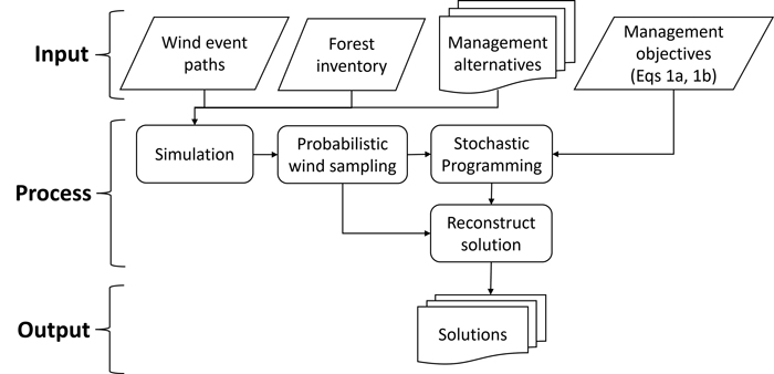
Fig. 1. Workflow of the study including the input information about wind, forest, and management and the modelling process used to find the final solutions.
2.2 Input
2.2.1 Forest inventory
The forest holding is in the municipality of Korsnäs (western Finland), near the Gulf of Bothnia (Fig. 2 and Supplementary file S1). This region of Finland is known for its frequent high-speed winds. We extracted the forest inventory data from Metsään.fi, an open-access database documenting the state of forests across Finland. The forest holding is 287.5 ha, consisting of 286 forest stands (relatively homogenous parcels of forested land) with a mean area of 1 ha (± standard deviation of 1.19). The forest holding is dominated by Myrtillus and Calluna site types (Cajander 1926, 1949). The forest is relatively well stocked, with an average of 145.5 m3 ha–1 and an average dominant height of almost 16 m.
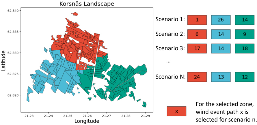
Fig. 2. A representation of the creation of the set of wind scenarios. For each zone, a wind event path (a set of wind events at varying intensities across the planning horizon) is selected, with a single landscape-level wind scenario being a combination of wind event paths for each zone.
2.2.2 Wind event paths
In our simulations, we defined a wind event path by its intensity (wind speed) and frequency (number of occurrences). To estimate potential wind risk, the wind event paths were included into the simulations as a large (but manageable) set of deterministic wind disturbances for the forest simulator. To construct a wind event path for each stand, we applied a set of predefined wind intensities at specific time intervals. To limit the number of potential wind event paths, we limited the range of wind speeds and return frequency. For wind speed, we used three intensity levels: low (14 m s–1), moderate (18 m s–1) and high (22 m s–1) wind speeds. We limited the return frequency depending on the intensity of the wind. The allowed combinations of intensity and frequency were restricted using a simple algorithm. The algorithm used a point system to manage how often strong winds would happen across the simulations. Each wind event was allocated points based on its strength: 1 for low, 2 for moderate and 3 for high intensity. We allowed a maximum of 4 points in total, meaning the simulation could include only one high intensity or two moderate storms over the planning horizon. We limited high intensity wind disturbances due to the significant damage they inflict, leading to little possible damage if a second high intensity wind disturbance would occur. Even with these simplifications, we generated a large set of deterministic wind event paths (204, Suppl. file S2). These can be used as input data for a stochastic programming formulation incorporating wind risk. The simplification of the wind event paths also facilitated easier interpretation of the optimization results.
2.2.3 Management alternatives
A specific set of management alternatives was constructed for each stand. We developed these management alternatives using a branching approach (Siitonen 1993) applied to the simulated case with no wind events. The management actions included in the branching process encompasses processes relevant to rotation forestry, a dominant management type in Finland: thinning, selective harvesting and final felling followed by regeneration actions. The number of forest management alternatives varied per stand, ranging from 1 to 19 with an average of 6.5 and a standard deviation of 3.8. The quantity of management alternatives depends on the initial conditions of the forest stand and what actions are possible during the planning horizon.
We applied the same set of management alternatives to each wind event path. In the case where a forest silvicultural action could not be executed due to significant wind damage, no silvicultural actions were applied. We assumed that after a wind damage event, salvage operations would occur in the same period, with the salvaged timber sold to the market. To ease the complexity of the model, we held timber prices and salvage prices constant across the planning horizon. The timber prices we selected mirror the current market prices in 2023. Salvage timber price was assumed to be 15 € m–3. This price was assumed to include salvage costs and accounts for the proportion of salvageable wood and quality of the wood salvaged. To test the impact of differing salvage prices we conducted a sensitivity analysis using salvage timber prices of 5, 10, 15 and 20 € m–3, found in the interactive binder hyperlink from the data and code availability section.
2.3 Process
2.3.1 Simulation
Forest simulations were conducted using the SIMO forest simulator (Rasinmäki et al. 2009). This simulator consists of a package of over 400 forest models to project the development of the forest over time, providing a range of economic and ecological indicator values. To focus on near term planning decisions, a planning horizon of thirty years (six 5-year periods) was used.
To account for potential wind damage in the forest simulation, we used the HWind model (Peltola et al. 1999). This model estimates the critical wind speeds required to fell trees in the forested stand. We employed a specific variant of the HWind model based on the revisions by Heinonen et al. (2009). To limit the spatial effects of the neighboring stands trees, we assumed a constant height of 10 m for the neighboring stand.
2.3.2 Probabilistic wind sampling
We generated wind scenarios by applying a Monte Carlo sampling approach to select a wind event paths from each zone in the landscape. To reflect frequency and intensity patterns we restricted the choice of wind event paths to specific groups based on their frequency and intensity. Each grouping contained sets of wind event paths from which we drew samples to represent wind scenarios. We created five groups: low intensity and low frequency (LL), low intensity and high frequency (LH), moderate intensity and low frequency (ML), moderate intensity and moderate frequency (MM) and high intensity and low frequency (HL), with the description of groupings in Table 1. Some combinations, such as high intensity and high frequency, or high intensity and moderate frequency, were not possible as we only allowed for one high intensity wind events across the planning horizon. For a detailed description of the intensity and specific timing of the wind events, see Suppl. file S2.
| Table 1. Allocation scheme that assigns wind event paths into a specific group that represents a specific set of intensities and frequencies. A wind event path is a set of wind events at varying intensities across the planning horizon. The five groups represent different assumptions of wind disturbance patterns: low intensity low frequency (LL), low intensity and high frequency (LH), moderate intensity and low frequency (ML), moderate intensity and moderate frequency (MM) and high intensity and low frequency (HL). Points from 1 to 3 were assigned to different wind intensities to regulate the frequency of wind disturbances, with a maximum of 4 points allowed per wind event path. | ||
| Number of wind event path (Total cases) | Point sum | Group (Intensity, Frequency) |
| No wind disturbance (1) | 0 | LL |
| 1 low intensity disturbance (6) | 1 | LL |
| 2 low intensity disturbances (15) | 2 | LL |
| 1 medium intensity disturbance (6) | 2 | ML |
| 3 low intensity disturbances (20) | 3 | LL |
| 1 high intensity disturbance (6) | 3 | HL |
| 1 low and 1 medium intensity disturbances (30) | 3 | ML |
| 1 low and 1 high intensity disturbances (30) | 4 | HL |
| 2 low and 1 medium intensity disturbances (60) | 4 | ML |
| 2 medium intensity disturbances (15) | 4 | MM |
| 4 low intensity disturbances (15) | 4 | LH |
For this case study, a specific wind disturbance group (out of the 5 groups described above) can be assigned to a specific zone of the forest holding. The justification for this is to allow for wind event paths to occur in spatially distinct regions across time, as a wind event path can occur in spatially specific zones and across entire landscapes. These regions split the forest holding into three zones, each being assigned a random wind event path (from the wind disturbance group). This is presented graphically in Fig. 2, where for each wind scenario, each zone is assigned a unique wind event path. To ease the simulation, we assumed that the storm affects all stands in the zone. While this is a simplification of reality, it highlights how increasingly realistic wind risk scenarios could be generated for use in stochastic programming formulations. Following the optimization, we re-applied this approach, to assess how well the solution performs when using different assumptions of wind.
2.3.3 Stochastic programming formulation
We apply a stochastic programming formulation that strives to balance between maximization of the economic value of the forest (the net present value) and periodic timber extraction from the forest to provide a relatively even flow of income and supply of timber to mills, measured using the CvaR (Rockafellar and Uryasev 2000). The CVaR quantifies the average loss exceeding the Value at Risk (VaR) at α% from the distribution of outcomes. The parameter α is selected by the decision maker and reflects the risk preferences of the individual. The VaR corresponds with the α% outcome however optimizing for VaR is non-linear (requiring integer programming to solve), while the CVaR can be linearized, simplifying the computational demands of the optimization problem (Rockafellar and Uryasev 2000). This model strives to mitigate risk of meeting the even-flow requirements and can be re-ran by the decision maker to update the plan as needed once uncertainty becomes revealed. The problem formulation resembles single-stage stochastic programming models (Eyvindson and Cheng 2016). In this case, the first objective function (1a) maximizes the expected net present value (NPV), with the second objective function (1b) minimizing the maximum CVaR across all periods in the planning horizon. To ensure efficiency (to avoid internal optimums), both objective functions include the alternative augmented objective function. The augmentation term has a small coefficient, ρ, which ensures the augmentation part does not affect unless there is room for “free lunch”, meaning room for increasing the value of the second objective without any trade-offs with the first.
Objective functions:
![]()
![]()
Subject to:

![]()
![]()

![]()


where pn is the probability of the wind scenario n; NPVn is the net present value of the wind scenario n; E(NPV) is the expected value of the net present value; CVaR* is the maximum conditional value at risk from all periods evaluated using a confidence level of α; Int is the income generated during scenario n and period t; PVjkn is the estimated discounted future land and timber value (calculated using models of (Pukkala 2005)) from stand j and management schedule k for scenario n; r is a parameter describing the discount rate applied; CVaRt is the conditional value at risk for period t; xjk is the decision variable for stand j and management schedule k; P represents the value of the wood (w) for each assortment (a), salvage wood (s) and the costs (c) of silvicultural activities; Hajknt and Sjknt respectively represents the quantity of the assortment of timber or salvage material, stand j, management schedule k for wind risk scenario n at period t; Cjknt represents the silvicultural costs for the stand j, management schedule k for wind scenario n at period t; Lnt is the downside losses (the deviations below the even-flow target for each time periods) for wind scenario n at period t; bt is the income target for each period t; Zt is the value at risk for period t. See Table 2 for a more readable description of these notations.
| Table 2. Notation used in the stochastic programming models. | |
| Symbol | Description |
| Sets | |
| N | The set of wind scenarios representing the forest holding level uncertainty |
| T | The set of time periods under consideration |
| J | The set of stands representing the forest holding |
| Variables | |
| pn | The probability of a wind scenario n |
| CVaR* | The maximum conditional value at risk from all periods evaluated using a confidence level of α |
| CVaRt | The conditional value at risk for period t |
| E(NPV) | The expected net present value for the set of wind scenarios |
| Hajknt | The quantity of wood for the specific assortment a, at stand j, for management schedule k, for wind risk scenario n, at period t |
| Int | The income generated during wind scenario n and period t |
| Lnt | The downside losses for wind scenario n and period t |
| NPVn | The net present value of a wind scenario n |
| PVjkn | The remaining productive value from stand j and management schedule k for wind scenario n |
| xjk | The decision variable for stand j and management schedule k |
| Sajknt | The quantity of salvage material for wind scenario n, stand j, management schedule k, and period t |
| Zt | The value at risk for period t |
| Parameters | |
| bt | The income target for each period t |
| Cjknt | The silvicultural actions for stand j, management schedule k, wind risk scenario n, and period t |
| ρ | A small positive value to act as an augmentation term |
| P | The value of the assortment of timber, salvage wood, and the costs of silvicultural activities |
| r | A parameter describing the discount rate applied |
Eq. 1a is the objective function that maximizes E(NVP), and Eq. 1b minimizes the maximum CVaR. By minimizing the maximum CVaR, the focus of the objective function is to ensure all deviations from the highest possible periodic harvest level is as small as possible. Both objective functions include an augmentation term, ρ set to 0.0001 for Eq. 1a and 0.0000001 for Eq. 1b, ensuring the solution’s efficiency with respect to the alternative indicator. Eq. 2 computes the net present value for each scenario, while Eq. 3 evaluates the E(NVP). Eq. 4 assesses the maximum CVaR for each time period in T, and Eq. 5 measures the income generated for each scenario within a specific period. Eq. 6 evaluates the negative deviations from the specific income target (bt), while Eq. 7 assesses the conditional value at risk for each period. The square brackets in Eqs. 6 and 7 implies that only positive values are considered, and any negative value will be set to 0. Finally, Eq. 8 ensures the entire stand is managed according to a specific treatment schedule, aligning with the Model I formulation from Johnson and Scheurman (1977). For this case study, we set the income target (bt) at 75% of the maximum possible sustained harvest income (specifically 700 € ha–1 year–1), as this target could be reached under most wind scenarios.
2.4 Output
Once a solution (a specific set of treatment decisions for each stand in the landscape) was found for the specific optimization problem, we applied the set of obtained decisions to a new set of Monte Carlo simulations for each wind disturbance group (i.e. LL, LH, ML, MM, HL). We used the same sampling scheme as described earlier in “Probabilistic wind sampling” section.
This process generates a dataset that applies the solutions derived from the stochastic programming problem. This approach was used for two main reasons: to remove the perception of anticipatory planning just prior to serious wind disturbance, and to reduce the number of apparent artifacts in the results presentation. In a stochastic programming, anticipatory planning refers to using information about the future that might not be available until after the disturbance has occurred. While this issue is significant in multi-staged stochastic programming, it is less problematic in single-staged stochastic programming as we used here, where scenarios represent the probability of occurrence. Presenting the direct results obtained stochastic programming solution may include artifacts from the optimization process. These artifacts could be presented as exact income target for the periodic income, which is highly unlikely in stochastic processes. For the case when minimizing the CVaR (the maximum conditional value at wind risk from all periods), the results can fall exactly at the harvesting target. This can be seen as an extreme occurrence, obtained by optimizing for the sample scenario set. By applying the solution to a new sample scenario set, we can get a more representative outcome.
3 Results
These results highlight the potential benefits of accurately predicting wind intensity and frequency, as well as the potential challenges when the predictions of wind do not match the ‘real’ occurrence of wind. This is seen in Fig. 3 where we contrast the performance of optimized solution for a specific wind scenario with the occurrence of all the wind scenarios. To simplify the portrayal of the results, we will focus on comparing the decisions made for the two most contrasting sets of scenarios: low intensity and low frequency wind risk cases (LL) and the high intensity and low frequency wind risk cases (HL). This quantifies the difference in the planning outcomes from using correct and incorrect assumptions of wind uncertainty used for decision making. Additional comparisons of all other wind risk cases can be found in the interactive online graphing tool with the link found in the data and code availability section.
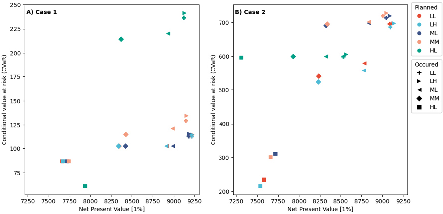
Fig. 3. A scatter plot of the two objectives (expected net present value (E(NPV)) (x-axis) and the minimum conditional value at risk (CvaR)) values across all 6 periods. Panel A) represents the cases when Equation 1A (maximizes E(NPV)) is the objective function, Panel B) represents the case when Equation 1B (minimizes the maximum CVaR). The colors represent the wind scenario assumption made when planning, while the marker represents the possible occurrence of a specific wind risk scenario. Note different scale on y-axes. View larger in new window/tab.
Case 1 – Objective function 1a, maximizing the expected net present value:
When our objective is to maximize E(NVP), forest stands are generally harvested rather rapidly once they reach economic maturity. Each solution for their respective assumption yields the largest E(NVP) (Fig. 4A, Table 3). However, there are notable differences between the performance of planning for correct vs incorrect wind risk assumptions. If we plan for the high intensity low frequency (HL) wind scenario set when the low intensity low frequency (LL) set of wind scenarios occurs, there is a 1 % reduction in the NPV. In contrast there is a 3.5% reduction in the NPV if we plan for the LL set of wind scenarios and the HL wind scenarios occurs (Table 3). The main difference in the planned decisions lies in the shift towards earlier timber harvesting when we assume that the HL set of wind scenarios case will occur. This shift reduces the expected value of the forest stand as wind risk probabilities increase. Conversely, if low wind risk is assumed (LL or LH), trees are left to grow longer on the stand. This logic aligns with the results of other studies exploring the impact of natural hazards on forests (Diaz-Balteiro et al. 2014). It emphasizes that overly optimistic assumptions about the wind risk can incur substantial economic costs (when planning is based on low wind risks). On the other hand, pessimistic assumptions result in lower economic costs (when planning is based on high wind risks). To allow for a comparison with case 2, we provide the distribution of the periodic incomes in Suppl. files S3 and S4.
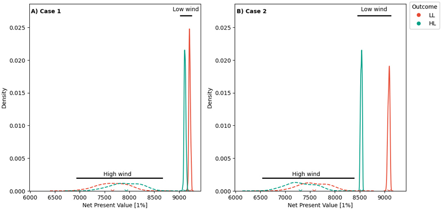
Fig. 4. The performance of the expected net present value (E(NPV)) for both cases. Case 1: is when we aim to maximize the E(NPV), while case 2 we aim to minimize the maximum conditional value at risk (CVaR). The solid lines represent the case when low intensity low frequency (LL) wind scenarios occur, while the dashed lines represent the case when high intensity low frequency (HL) wind scenarios occur. The red lines (LL) represent that planning is based on the assumption for the LL wind scenarios occur, while the green (HL) lines represent that planning is based on the assumption is the HL wind scenarios occur. View larger in new window/tab.
| Table 3. Comparison of the optimized solutions, either maximizing expected net present value (E(NPV)) or minimizing the conditional value at risk (CVaR). The payoff table describes the specific cases depending on which wind patterns are planned for versus if a different wind pattern would occur, where LL stands for low intensity low frequency wind and HL – high intensity low frequency wind. | ||||||
| MAX E(NPV) | MIN CVAR | |||||
| LL Occurs | HL Occurs | LL Occurs | HL Occurs | |||
| E(NPV) | Planned for LL | 9214 | 7657 | 9087 | 7578 | |
| Planned for HL | 9119 | 7933 | 8 535 | 7304 | ||
| CVAR | Planned for LL | Period 1 | 1774 | 1703 | 1218 | 1211 |
| Period 2 | 677 | 486 | 697 | 494 | ||
| Period 3 | 410 | 216 | 699 | 446 | ||
| Period 4 | 113 | 87 | 696 | 338 | ||
| Period 5 | 443 | 214 | 698 | 435 | ||
| Period 6 | 462 | 130 | 699 | 235 | ||
| CVAR | Planned for HL | Period 1 | 1944 | 1853 | 599 | 599 |
| Period 2 | 808 | 577 | 995 | 599 | ||
| Period 3 | 279 | 219 | 994 | 620 | ||
| Period 4 | 237 | 122 | 809 | 613 | ||
| Period 5 | 590 | 271 | 953 | 610 | ||
| Period 6 | 297 | 61 | 1018 | 597 | ||
Case 2 – Objective function 1b, minimizing the maximum CVaR:
When we shift the priority from maximizing E(NVP) to minimizing the maximum CVaR across all planning periods, there is a slight decrease in the E(NVP) when correctly assuming the LL wind scenarios (Fig. 4B and Table 3). Minimizing CVaR results in a reduction of the maximum NPV obtained by 1.4%. In contrast, when correctly assuming a high wind risk scenario (HL), the required reduction in E(NVP) to minimize the maximum CVaR is dramatically higher (7.9%). The CVaR* for the high wind risk scenario (HL) is considerably higher than for the low wind risk scenario (LL). This difference can be attributed to the challenge of meeting the selected harvest target while expecting a high-intensity wind path (Figs. 5 and 6).
For the case when the assumption regarding which wind risk scenario would occur was incorrect, there were dramatic impacts to the expected outcomes. In the case where we assume high wind risk (HL) but low wind (LL) occurs, proactively managing the forest for high wind risks can lead to a considerable reduction in the E(NVP) (7.9%) and significant overshooting of the harvest income target for all periods except the first period. When planning for high wind disturbance events, there is an expectation that a large component of the income comes from salvage harvest operations, across all planning periods. With less wind disturbance events than expected, there will be little salvaged wood in the first period, and planned operations in subsequent periods will include a buffer anticipating that some stands will have been affected by wind disturbance. The specific income obtained from the salvaged timber will depend on quality of the salvage material, which can be explored in the sensitivity analysis (see the data and code availability section). On the other hand, ignoring the potential for high wind risks slightly improves the E(NVP) (with a 3.8% increase). However, it severely impacts the ability to collect stable income from the forest. For all except the first period, the median harvested per hectare income is less than the target, with the CVaR at 5% having a range between 235 € ha–1 and 494 € ha–1.
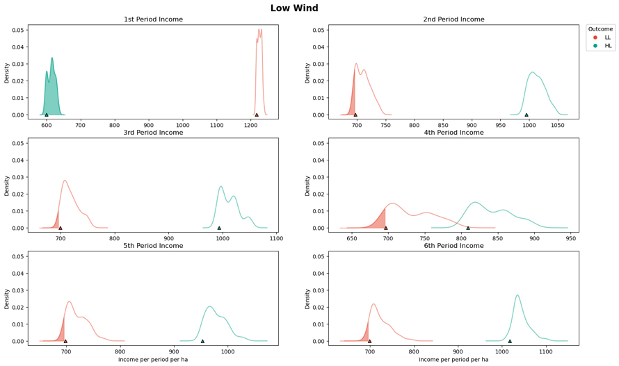
Fig. 5. The period incomes for the case when minimizing the maximum conditional value at risk (CVaR) (Case 2) when low intensity low frequency wind scenarios occur (LL). The solid red lines present the periodic incomes when planning for the low intensity low frequency (LL) wind scenarios (correct assumption). The solid green (HL) lines present the periodic incomes when planning for the high intensity low frequency wind scenarios. The shaded area of the graph indicates when the targeted income value has not been met, with the symbol at the x-axis corresponds to the CVaR value. View larger in new window/tab.
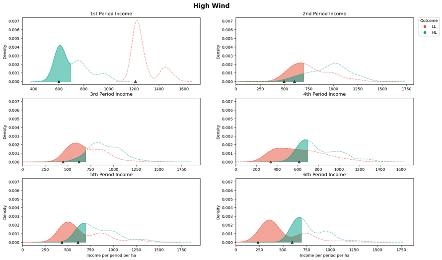
Fig. 6. The period incomes for the case when minimizing the maximum conditional value at risk (CVaR) (Case 2) when high intensity low frequency wind scenarios occur (HL). The dotted red lines (LL) present the periodic incomes when planning for the low frequency low intensity (LL) wind scenarios. The dotted green (HL) lines present the periodic incomes when planning for the high intensity low frequency wind scenarios (correct assumption). The shaded area of the graph indicates when the targeted income value has not been met, with the symbol at the x-axis corresponds to the CVaR value. View larger in new window/tab.
For interested readers we have constructed an interactive software package to explore and compare the other scenarios. Information is provided in the data and code availability section section.
4 Discussion
This study has demonstrated a stochastic programming approach to incorporate wind risk into the planning process. To appropriately mitigate the impacts of wind disturbances, we must first establish what aspect of risk is to be mitigated. We explore risk as the negative consequences that occur to the decision makers’ objective function (Eyvindson and Kangas 2018). Thus, we focus not to minimize the impacts of the disturbance, but on the impacts to the desires of the decision maker. In this study, we explored two facets of risk. Firstly, we examined the risk to E(NPV) as illustrated in Eq 1a. Secondly, we looked at the risk associated with achieving a sustainable harvesting target across all planning periods, as measured by the CVaR in Eq. 1b.
In the pursuit of maximizing the expected value of NPV, we found only a minor advantage in incorporating wind risk into the planning process. This result may appear to conflict with earlier studies that aim to minimize the potential effect of wind. For instance, Ruotsalainen et al. (2023) compared the impact of optimizing for NPV and minimizing the weighted canopy height difference, with canopies having less height differences implying less risk. They evaluated risk as the number or area of trees likely to be felled by wind at varying speeds. Minimizing canopy height differences effectively reduces the probability of trees being felled by strong winds, albeit at a large economic cost. Using stochastic programming, we modify the impact of wind risk which is directly linked to the probability of a sufficiently intense storm to cause damage to the forest stand. Maximizing the E(NPV) includes a risk mitigation component, as forest stands are harvested once they are mature, leaving very little time for the forest stand to be impacted by wind.
Contrarily, when minimizing the CVaR to meet specific periodic harvest objectives, stochastic programming can have a substantial impact to mitigate the damage caused by wind. For this case we applied a relatively high target for the sustainable extraction of timber (~75% of the case when no wind risk is assumed). Achieving and maintaining the target of sustained timber harvests was manageable for the low intensity low frequency wind scenario, however this was not the case for the high intensity low frequency scenario. For the case when timber harvest can be attained, the CVaR is nearly at (or above) the targeted harvest. The reason why the CVaR is not always above the harvest target is due to the difference between the scenarios used in the optimization and scenarios used to evaluate the results of the solutions. For both cases, the CVaR was evenly distributed across all periods (Figs. 5 and 6).
The cases presented in the results and Suppl. file S1 represent a variety of wind scenarios. Regardless of which scenarios were considered, all scenarios performed reasonably when maximizing NPV, with differences in NPV within a 1% to 3% range (Fig. 3, panel A). The results showed a consistent pattern: the larger the disparity is between the planned scenario and the actual wind scenario, the larger the impact is on the resulting NPV. When minimizing the CVaR, the solutions’ ability to meet the income target varied substantially. For low intensity wind scenarios (LL and LH), the performance limiting the CVaR suffered dramatically under higher intensity wind scenarios (MM, ML and HL) (Fig. 3). Only the high intensity, low frequency planning case performed well across the range of wind scenarios, maintaining a relatively constant minimum CVaR (at about 600 € ha–1 period–1) with only a moderate impact on the NPV. This strategy may be applied by a risk averse decision maker, who pessimistically plans for the worst possible future outcomes.
Despite the complexity of this approach, the technical challenges are not dramatically greater than those of standard deterministic forest planning approaches. This method requires re-simulation of the landscape a total of 204 times to account for various wind event paths. Although this does dramatically increase the number of simulations, the increase is not exponential, unlike in multi-staged stochastic programs (Eriksson 2006), and can be managed without requiring excessive computational power. Once logical wind simulations are constructed, generating potential wind scenarios is straightforward. This just requires replicating variations of the development of the forest according to projections of wind occurrence at the landscape scale.
While we explore only a single natural disturbance, the approach could be extended to address multiple disturbances through a similar framework and can explore risks associated with various objective functions. The decisions taken must be able to influence either the disturbance probability or the effect it has on the decision makers objectives. In the cases where the disturbance probabilities cannot be impacted without additional information, inclusion of updated information is possible, and can be accomplished through two staged or multi-staged stochastic programming (Boychuk and Martell 1996; Eyvindson et al. 2017).
This study introduces a quantitative approach that integrates wind disturbances into forest planning processes. We present a practical approach to quantify and assess the potential risk of winds, enabling an assessment of the impact of wind. However, there remains a variety of issues to be resolved in future research. Forest disturbances, and wind especially can be impacted by the spatial configuration of the forest stands and the wind patterns dynamics. Some of these issues could be addressed through the use of heuristics or non-linear optimization (see Heinonen et al. 2011), and through improvements in how wind directions are incorporated into the simulations. Further work is additionally required to formulate multi-objective decision problems while enabling risk mitigation, and/or recognizing the potential benefits of disturbances, such as increased deadwood. In this way, further research can pave the way for more resilient forest management strategies that address risks in a proactive fashion.
5 Conclusions
To effectively minimize the impact of wind risk, decision makers must first identify which aspect of risk is to be minimized. In this study, we developed an approach to integrate wind disturbances into a stochastic programming framework. We specifically aimed to minimize the risk related to the even-flow harvest constraint, evaluated as the conditional value at risk (CVaR). With a similar approach, a wide variety of other risk aspects could be explored. While stochastic programming approaches are more computationally demanding than standard linear programming approaches, stochastic programming allows for the exploration into how uncertainty can be handled, and quantifies the main challenges relatating to forest simulations and optimization approaches. This extra effort opens up numerous opportunites to assess, quantify and mitigate impacts of risk in forest planning.
Data and code availability
The code to re-construct the analysis can be found at github.com: https://github.com/eyvindson/WindRiskGraphing. The simulation databases (a total of 6.45 Gb), the summarization of the key simulated information (a total of 1.15 Gb) and an archived version of the software can be found at the Zenodo repository: https://doi.org/10.5281/zenodo.8192110. To construct visualizations readers are directed to the Web Binder: https://mybinder.org/v2/gh/eyvindson/WindRiskGraphing/HEAD?labpath=INTERACT.ipynb.
Author contributions
KE created the software, wrote the original draft, conducted the visualization; KE and MP conceptualized the idea and performed the data curation; KE, JH-F, ON and MP conducted the formal analysis; KE and AK developed the methodology; and all authors contributed to the investigation of the ideas and writing review & editing of the manuscript.
Acknowledgements
We wish to thank CSC - IT Center for Science LTD for providing the high-performance computational resources.
Funding
We would like to acknowledge funding support from the Norwegian Research Council (NFR project 302701 Climate Smart Forestry Norway) and by the Academy of Finland Flagship UNITE (337653).
References
Birge JR, Louveaux F (2011) Introduction to stochastic programming. Springer New York, New York, NY. https://doi.org/10.1007/978-1-4614-0237-4.
Boychuk D, Martell D (1996) A Multistage Stochastic Programming Model for Sustainable Forest-Level Timber Supply Under Risk of Fire. For Sci 42: 10–26. https://doi.org/10.1093/forestscience/42.1.10.
Buongiorno J, Zhou M, Johnston C (2017) Risk aversion and risk seeking in multicriteria forest management: a Markov decision process approach. Can J For Res 47: 800–807. https://doi.org/10.1139/cjfr-2016-0502.
Cajander A (1926) The theory of forest types. Acta For Fenn 29. https://doi.org/10.14214/aff.7193.
Cajander A (1949) Forest types and their significance. Acta For Fenn 56. https://doi.org/10.14214/aff.7396.
Dantzig GB (1998) Linear programming and extensions. Princeton University Press, Princeton, NJ.
de Pellegrin Llorente I, Eyvindson K, Mazziotta A, Lämås T, Eggers J, Öhman K (2023) Perceptions of uncertainty in forest planning: contrasting forest professionals’ perspectives with the latest research. Can J For Res 53: 391–406. https://doi.org/10.1139/cjfr-2022-0193.
Diaz-Balteiro L, Martell DL, Romero C, Weintraub A (2014) The optimal rotation of a flammable forest stand when both carbon sequestration and timber are valued: a multi-criteria approach. Nat Hazards 72: 375–387. https://doi.org/10.1007/s11069-013-1013-3.
Eriksson LO (2006) Planning under uncertainty at the forest level: a systems approach. Scand J For Res 21: 111–117. https://doi.org/10.1080/14004080500486849.
Eyvindson K, Cheng Z (2016) Implementing the conditional value at risk approach for even-flow forest management planning. Can J For Res 46: 637–644. https://doi.org/10.1139/cjfr-2015-0270.
Eyvindson K, Kangas A (2014) Stochastic goal programming in forest planning. Can J For Res 44: 1274–1280. https://doi.org/10.1139/cjfr-2014-0170.
Eyvindson K, Kangas A (2016) Evaluating the required scenario set size for stochastic programming in forest management planning: incorporating inventory and growth model uncertainty. Can J For Res 46: 340–347. https://doi.org/10.1139/cjfr-2014-0513.
Eyvindson K, Kangas A (2018) Guidelines for risk management in forest planning – what is risk and when is risk management useful? Can J For Res 48: 309–316. https://doi.org/10.1139/cjfr-2017-0251.
Eyvindson KJ, Petty AD, Kangas AS (2017) Determining the appropriate timing of the next forest inventory: incorporating forest owner risk preferences and the uncertainty of forest data quality. Ann For Sci 74, article id 2. https://doi.org/10.1007/s13595-016-0607-9.
Filippi C, Mansini R, Stevanato E (2017) Mixed integer linear programming models for optimal crop selection. Comput Oper Res 81: 26–39. https://doi.org/10.1016/j.cor.2016.12.004.
Forsell N, Wikström P, Garcia F, Sabbadin R, Blennow K, Eriksson LO (2011) Management of the risk of wind damage in forestry: a graph-based Markov decision process approach. Ann Oper Res 190: 57–74. https://doi.org/10.1007/s10479-009-0522-7.
Gardiner B, Byrne K, Hale S, Kamimura K, Mitchell SJ, Peltola H, Ruel J-C (2008) A review of mechanistic modelling of wind damage risk to forests. Forestry 81: 447–463. https://doi.org/10.1093/forestry/cpn022.
Heinonen T, Pukkala T, Ikonen V-P, Peltola H, Venäläinen A, Dupont S (2009) Integrating the risk of wind damage into forest planning. For Ecol Manag 258: 1567–1577. https://doi.org/10.1016/j.foreco.2009.07.006.
Heinonen T, Pukkala T, Ikonen V-P, Peltola H, Gregow H, Venäläinen A (2011) Consideration of strong winds, their directional distribution and snow loading in wind risk assessment related to landscape level forest planning. For Ecol Manag 261: 710–719. https://doi.org/10.1016/j.foreco.2010.11.030.
Johnson KN, Scheurman HL (1977) Techniques for prescribing optimal timber harvest and investment under different objectives – discussion and synthesis. Forest Science 23.
Kallio M, Kuula M, Oinonen S (2012) Real options valuation of forest plantation investments in Brazil. Eur J Oper Res 217: 428–438. https://doi.org/10.1016/j.ejor.2011.09.040.
Kangas A, Kurttila M, Hujala T, Eyvindson K, Kangas J (2015) Decision support for forest management. Springer Cham. https://doi.org/10.1007/978-3-319-23522-6.
King AJ, Wallace SW (2012) Modeling with stochastic programming. Springer New York, New York, NY. https://doi.org/10.1007/978-0-387-87817-1.
Kleywegt AJ, Shapiro A, Homem-de-Mello T (2002) The sample average approximation method for stochastic discrete optimization. SIAM J Optim 12: 479–502. https://doi.org/10.1137/S1052623499363220.
Palma CD, Nelson JD (2009) A robust optimization approach protected harvest scheduling decisions against uncertainty. Can J For Res 39: 342–355. https://doi.org/10.1139/X08-175.
Patacca M, Lindner M, Lucas‐Borja ME, Cordonnier T, Fidej G, Gardiner B, Hauf Y, Jasinevičius G, Labonne S, Linkevičius E, Mahnken M, Milanovic S, Nabuurs G, Nagel TA, Nikinmaa L, Panyatov M, Bercak R, Seidl R, Ostrogović Sever MZ, Socha J, Thom D, Vuletic D, Zudin S, Schelhaas M (2023) Significant increase in natural disturbance impacts on European forests since 1950. Glob Change Biol 29: 1359–1376. https://doi.org/10.1111/gcb.16531.
Peltola H, Kellomäki S, Väisänen H, Ikonen V-P (1999) A mechanistic model for assessing the risk of wind and snow damage to single trees and stands of Scots pine, Norway spruce, and birch. Can J For Res 29: 647–661. https://doi.org/10.1139/x99-029.
Potterf M, Eyvindson K, Blattert C, Burgas D, Burner R, Stephan JG, Mönkkönen M (2022) Interpreting wind damage risk–how multifunctional forest management impacts standing timber at risk of wind felling. Eur J For Res 141: 347–361. https://doi.org/10.1007/s10342-022-01442-y.
Pukkala T (ed) (2002) Multi-objective Forest Planning. Springer Netherlands, Dordrecht. https://doi.org/10.1007/978-94-015-9906-1.
Pukkala T (2005) Metsikön tuottoarvon ennustemallit kivennäismaan männiköille, kuusikoille ja rauduskoivikoille. [Prediction models for the expectation value of pine, spruce and birch stands on mineral soils]. Metsätieteen Aikakauskirja 3/2005: 311–322. https://doi.org/10.14214/ma.5778.
Rasinmäki J, Mäkinen A, Kalliovirta J (2009) SIMO: An adaptable simulation framework for multiscale forest resource data. Comput Electron Agric 66: 76–84. https://doi.org/10.1016/j.compag.2008.12.007.
Rockafellar RT, Uryasev S (2000) Optimization of conditional value-at-risk. J Risk 2: 21–41. https://doi.org/10.21314/JOR.2000.038.
Rönnqvist M, D’Amours S, Weintraub A, Jofre A, Gunn E, Haight RG, Martell D, Murray AT, Romero C (2015) Operations Research challenges in forestry: 33 open problems. Ann Oper Res 232: 11–40. https://doi.org/10.1007/s10479-015-1907-4.
Ruotsalainen R, Pukkala T, Ikonen V-P, Packalen P, Peltola H (2023) Mitigating the risk of wind damage at the forest landscape level by using stand neighbourhood and terrain elevation information in forest planning. For Int J For Res 96: 121–134. https://doi.org/10.1093/forestry/cpac039.
Siitonen M (1993) Experiences in the use of forest management planning models. Silva Fenn 27: 167–178. https://doi.org/10.14214/sf.a15670.
Suvanto S, Peltoniemi M, Tuominen S, Strandström M, Lehtonen A (2019) High-resolution mapping of forest vulnerability to wind for disturbance-aware forestry. For Ecol Manag 453, article id 117619. https://doi.org/10.1016/j.foreco.2019.117619.
Thom D, Seidl R (2016) Natural disturbance impacts on ecosystem services and biodiversity in temperate and boreal forests. Biol Rev 91: 760–781. https://doi.org/10.1111/brv.12193.
Wei Y, Bevers M, Nguyen D, Belval E (2014) A spatial stochastic programming model for timber and core area management under risk of fires. For Sci 60: 85–96. https://doi.org/10.5849/forsci.12-124.
Zeng H, Pukkala T, Peltola H (2007) The use of heuristic optimization in risk management of wind damage in forest planning. For Ecol Manag 241: 189–199. https://doi.org/10.1016/j.foreco.2007.01.016.
Zhou M, Buongiorno J (2019) Optimal forest management under financial risk aversion with discounted Markov decision process models. Can J For Res 49: 802–809. https://doi.org/10.1139/cjfr-2018-0532.
Zhou S, Erdogan A (2019) A spatial optimization model for resource allocation for wildfire suppression and resident evacuation. Comput Ind Eng 138, article id 106101. https://doi.org/10.1016/j.cie.2019.106101.
Zubizarreta-Gerendiain A, Pukkala T, Peltola H (2017) Effects of wind damage on the optimal management of boreal forests under current and changing climatic conditions. Can J For Res 47: 246–256. https://doi.org/10.1139/cjfr-2016-0226.
Total of 42 references.
Send to email
