Zsofia Koma  ,
Johannes Breidenbach
,
Johannes Breidenbach
Large-scale validation of forest attribute maps across different spatial resolutions
Koma Z., Breidenbach J. (2025). Large-scale validation of forest attribute maps across different spatial resolutions. Silva Fennica vol. 59 no. 2 article id 24061. https://doi.org/10.14214/sf.24061
Highlights
- The study assesses stand-level uncertainty of biomass, volume, basal area, and Lorey’s height estimates resulting from the prediction of maps across varying spatial resolutions (1–30 m)
- The changes of RMSE and bias across the different spatial resolutions were generally small (< 5%) for additive forest attributes such as biomass, volume, and basal area
- The changes of RMSE and bias were also small for Lorey’s height as a non-additive forest attribute if the resolution difference was less than 2 times of the native resolution
- The models fitted at the resolution of the NFI plot size can be used to produce forest attribute maps at 10 m resolution without concerning increases in uncertainty at stand-level.
Abstract
Fine-scale, spatially explicit forest attribute maps are essential for guiding forest management and policy decisions. Such maps, based on the combination of National Forest Inventory (NFI) and remote sensing datasets, have a long tradition in the Nordic countries. Harmonizing the pixel size among national forest attribute maps would considerably improve the utility of the maps for users. However, the maps are often aligned with the NFI plot size, and the influence of creating these maps at different spatial resolutions (i.e. pixel sizes) is little studied. We assess the stand-level uncertainty (RMSE) of biomass, volume, basal area, and Lorey’s height estimates resulting from the aggregation of maps across varying spatial resolutions. Models fit at 16 m native resolution using more than 14 000 NFI plots were applied for predictions at pixels sizes (side lengths) of 1, 5, 10, 16, and 30 m. For independent validation, we used more than 600 field plots – that cover a total area of 24 ha and were clustered within 65 stands across Norway. For all attributes, the lowest RMSEs, ranging from 6.86% for Lorey’s height to 13.86% for volume, were observed for predictions at pixel sizes of 5 m to 16 m. The RMSE changes across resolutions were generally small (< 5%) for biomass, volume, and basal area. For Lorey’s height, changing the spatial resolution resulted in large RMSEs of up to 25%. Overall, our findings suggest that the main forest attributes can be mapped at a finer resolutions without complex adjustments.
Keywords
airborne laser scanning;
National Forest Inventory;
forest resource mapping;
resolution dependence
-
Koma,
Norwegian Institute for Bioeconomy Research (NIBIO), Division of Forest and Forest Resources, Department National Forest Inventory, Høgskoleveien 7, 1433 Ås, Norway
 https://orcid.org/0000-0002-0003-8258
E-mail
zsofia.koma@nibio.no
https://orcid.org/0000-0002-0003-8258
E-mail
zsofia.koma@nibio.no
-
Breidenbach,
Norwegian Institute for Bioeconomy Research (NIBIO), Division of Forest and Forest Resources, Department National Forest Inventory, Høgskoleveien 7, 1433 Ås, Norway
https://orcid.org/0000-0002-3137-7236
E-mail
johannes.breidenbach@nibio.no
Received 1 November 2024 Accepted 21 August 2025 Published 11 September 2025
Views 22704
Available at https://doi.org/10.14214/sf.24061 | Download PDF

Supplementary Files
1 Introduction
Forests play a crucial role in the bioeconomy, for climate change mitigation and biodiversity conservation (Thompson et al. 2009; Griscom et al. 2017; Dinerstein et al. 2019). Sustainable management practices require reliable information on forests’ status and future development to minimize trade-offs and maximize synergies among the various ecosystem goods and services. Forest management at local scales is traditionally informed by Forest Management Inventories (FMIs). In the Nordic countries, FMIs are predominantly conducted using the Area-Based Approach (ABA) (Næsset 2002; Hyyppä et al. 2008; Maltamo et al. 2014) which combines Airborne Laser Scanning (ALS) and a limited number of field plots to provide fine-scale information about forest stands (Næsset et al. 2004; Maltamo et al. 2021). Over the last decade, the availability of national ALS campaigns has enabled the development of national forest attribute maps by utilizing in-situ data from National Forest Inventories (NFIs) (Nord-Larsen and Schumacher 2012; Nilsson et al. 2017; Tuominen et al. 2017; Hauglin et al. 2021). This provides spatially explicit forest resource maps at a national scale (McRoberts et al. 2010; Kangas et al. 2018; Fassnacht et al. 2023). Consequently, the application of national forest attribute maps is increasingly considered in FMIs (Maltamo et al. 2021; Rahlf et al. 2021).
The sample plot size and spatial resolution of forest attribute maps are typically congruent in traditional FMIs (Næsset 2014). This is to avoid systematic errors due to the use of resolution-dependent predictor and response variables in regression models (Magnussen et al. 2016). A metric is considered resolution independent if averaging over a certain number of adjacent cells (or pixels) yields the same results as if the metric were computed for the whole area as a single cell (Packalen et al. 2019). ALS metrics such as mean height and proportion of echoes, meet the condition of resolution-independence. However, other metrics like height quantiles and the number of echoes above specific thresholds do not possess this property. Furthermore, response variables such as measures of mean and total quantity per areal unit, are additive and therefore resolution independent (Köhl et al. 2006). Examples of these include above-ground biomass, volume, and basal area. However, dominant and mean height, which are not additive, are sensitive to spatial resolution (Magnussen et al. 2016; Packalen et al. 2019). In real-world applications, a combination of resolution independent and dependent predictor and response variables are typically utilized in forest attribute mapping (Næsset 2002; Næsset et al. 2004).
The pixel size of national forest attribute maps often deviates, to a smaller or larger degree, from the size of the NFI field plots (Kangas et al. 2018). This discrepancy can be attributed primarily to two factors. Firstly, forest attributes in NFIs are frequently assessed using sample plots of varying sizes. For example, many NFIs use concentric sample plots or relascopes to select trees to be observed, where smaller trees are assessed on smaller circles than larger trees (Tomppo et al. 2008). Secondly, for large-scale applications, practical considerations related to data management and downstream analysis often influence the spatial resolution (Nilsson et al. 2017). For instance, circular plots with a size of 250 m2 as in the Norwegian NFI (Breidenbach et al. 2020), would require pixels with a side length of ca. 15.8114 m. A map with such a pixel size would be impractical on national scales as there will be no overlap with other existing mapping infrastructure.
While the analysis of resolution dependence in ABA is important, it remains a relatively underexplored field of study. Packalen et al. (2019) systematically identified factors and quantified effects on uncertainties with changing spatial resolutions when applying the ABA. Their study was conducted on a pine-dominated study-site in Finland where the biomass of all trees on 58 plots with a size of 25 m × 25 m was measured. This setup enabled various combinations of fitting and prediction at spatial resolutions across 8.33, 12.5, and 25 m pixel sizes. They found that if models with resolution-independent variables were used to predict at a finer resolution than the fitted (native) resolution, it resulted in a decrease of RMSE, and in tendency a systematic underestimation. If the models were applied at a coarser prediction resolution than the fitted resolution, it resulted in increased RMSE, and in tendency a systematic overestimation. They concluded that the resolution effect is minimal in the case of up to 4-times changes of the resolution. This suggests that in practical scenarios, a mismatch in spatial resolution between model fitting and applied prediction can be acceptable for forest attribute mapping. However, this study was conducted on a local site in Finland and focused solely on biomass. Nilsson et al. (2017) analyzed in Sweden the changes in random error for volume and Lorey’s height forest attributes across 10 m to 20 m resolutions. They found that, despite the native resolution of the Swedish forest resource map being 25 m based on the NFI plot size, the predicted maps with a resolution of 12.5 m were found to be satisfactory for producing the national forest attribute maps. Fassnacht et al. (2018) conducted a systematic analysis with varying plots and sample sizes (10–50 m) and estimated at various pixel sizes using synthetic remote sensing datasets. They observed small RMSE decrease with increasing plot sizes.
We aim to assess the uncertainty of the models used to create the Norwegian forest attribute map (Astrup et al. 2019; Hauglin et al. 2021) when applied across varying spatial resolutions. More specifically, we analyze the changes in uncertainty of models that were fitted at 16 m native resolution when applied to predict forest attributes for pixels with side lengths between 1 and 30 m. We aggregate the pixel-level predictions to stand-level estimates and analyze the resulting uncertainty for the forest attributes biomass, volume, basal area, and Lorey’s height. Independent field measurements of 65 stands widely distributed across Norway are used as a reference.
2 Materials and methods
2.1 Overview and study area
The Norwegian forest attribute map is a collection of spatially explicit raster layers with a pixel size of 16 m × 16 m which includes predicted forest attributes of biomass, volume, basal area, and Lorey’s height (Hauglin et al. 2021). The raster layers are generated from univariate linear mixed-effect models that utilize NFI data, country-wide ALS, and additional auxiliary data products. The map covers all forested areas in Norway, approximately 12 Mha, and is openly available at Kilden (NIBIO 2024).
Forests cover ca. 38% of Norway’s total land area and are predominantly situated in the boreal climate zone. The forests are dominated by three main tree species: Norway spruce, Scots pine, and deciduous trees, primarily birch, which are often mixed with the coniferous species. The country has a diverse topographical variation including both lowland and mountainous areas.
The independent field validation data used in this study are located across the whole of the country, including the South-Eastern, Central-Southern, Western, and Northern geographic regions (Fig. 1). Overall, 65 stands have been used with sizes ranging from 0.1 to 1.7 ha and an average of 0.4 ha. Altogether, the stands cover covers 24 hectares.
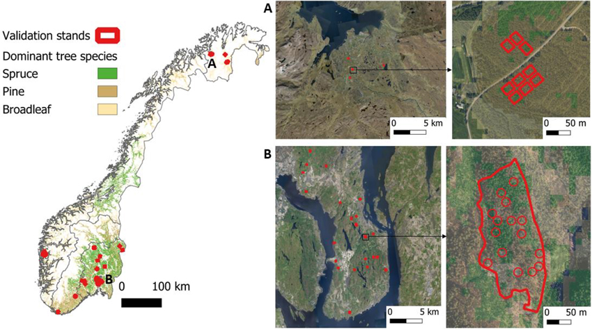
Fig. 1. Overview of the study area and the independent validation datasets. The left side is an overview map of Norway that shows the geographic regions (South-East, Central-South, West, Mid, and North) and the dominant tree species. Red polygons indicate the independent validation stands. The right side shows selected areas (A and B) in higher detail with orthophotos in the background. The maps are in the Universal Transverse Mercator (UTM) coordinate system zone 33. The dominant tree species map is from Kilden (NIBIO 2024), and orthophotos from Geonorge (2024).
Further details on the models used in producing Norwegian forest attribute maps, the independent field data, and the study design are given in sections 2.2, 2.3, and 2.4.
2.2 The Norwegian forest attribute map
2.2.1 National Forest Inventory data
The NFI is a continuously operating inventory based on a permanent sample grid where 1/5 of the plots are measured annually (Breidenbach et al. 2020). The sample grid size in productive forest is 3 km × 3 km. The NFI field measurements are carried out within circular 250 m2 plots. Diameter at breast height (dbh) and species of all trees with a dbh >= 5 cm are recorded. The height of ten trees are measured. Using these measurements together with species-specific models, missing tree heights, timber volume (with bark), and aboveground biomass are predicted for the trees at the sample plots. Tree-level measurements are scaled-up to plot-level values including Lorey’s height and basal area. More detailed information on the Norwegian NFI can be found in Breidenbach et al. (2020). The complied training data consists of 14 196 NFI plots from the inventory cycle 2018–2022.
2.2.2 Predictor variables
The predictor variables for estimating forest attributes are derived from country-wide ALS data. The ALS data were collected in national flight campaigns conducted by the Norwegian Mapping Agency, covering most of Norway except high mountainous regions (Hauglin et al. 2021). In this study the following predictor variables have been used: mean height of first returns (hmean_first in m), the square of the mean height of first returns (hmean_first_sq in m), proportion of first returns above 2 m (prop_ab2m_first in %) and 95th height percentile of first returns (h95_first in m). Additionally, the topographical slope (slope in degrees) has been calculated based on the 1 m × 1 m resolution digital terrain model. A further explanatory variable was the time difference between the ALS acquisition date and field date expressed as a decimal number of growth seasons (time_diff in days).
2.2.3 Regression models
The Norwegian forest attribute maps are generated as wall-to-wall predictions of univariate linear mixed-effects regression models (Pinheiro and Bates 2000). These models accommodate systematic differences between ALS projects (described in 2.2.1.) and regions by incorporating random effects. The regions are natural geographic divisions within Norway (Fig. 1). The predictor variables used in the models were selected through a stepwise process using leave-one-out cross-validation and expert knowledge, as described in Hauglin et al. (2021). In this study, we used the models to predict above-ground biomass, volume, basal area, and Lorey’s height. The models were fitted separately for each dominant tree species group (spruce, pine, and deciduous forests). The dominant tree species group for each NFI plot is determined by the tree species that has the largest proportion of the total volume. For prediction purposes, a wall-to-wall map (Breidenbach et al. 2021) is used to determine the dominant tree species across the country. The general form of the models is:

where yijk is the forest attribute at plot k within ALS project j and region i; r is the number of regions; p is the number of explanatory variables x; β are the fixed effects regression parameters and bi indicates a predicted random effect. Random slope parameters b for region i and b1 for ALS project area ij are defined as the most influential explanatory variable x1. The terms nij and mi represent the number of field plots within an ALS project and the total number of ALS projects respectively. The variance of the random effect is denoted by ![]() , and
, and ![]() refers to the residual variance. Four types of combinations of explanatory variables (introduced in section 2.2.2) have been used for predicting the species-specific forest attributes:
refers to the residual variance. Four types of combinations of explanatory variables (introduced in section 2.2.2) have been used for predicting the species-specific forest attributes:
i) For predicting biomass, volume and basal area for spruce and broadleaf forests: hmean_first (x1), + hmean_first_sq (x2), + time_diff (x3), + slope (x4), + prop_ab2m_first (x5),
ii) For predicting basal area for pine forests: hmean_first (x1), + hmean_first_sq (x2), + time_diff (x3), + prop_ab2m_first (x4),
iii) For predicting volume for pine forests: hmean_first (x1), + hmean_first_sq (x2), + time_diff (x3), + slope (x4),
iv) For predicting Lorey’s height for spruce, pine and broadleaf forests: h95_first (x1), + time_diff (x2), + slope (x3), + prop_ab2m_first (x4).
The predictor variables are resolution-independent in the case of hmean_first, hmean_first_sq, and prop_ab2m_first assuming the number of echoes per cell is constant. The variable h95_first is a resolution-dependent predictor variable since height percentiles are not unbiased corresponding to the population parameters (Magnussen et al. 2016; Packalen et al. 2019). Additionally, the slope is also a resolution-independent predictor variable.
2.3 Validation stands
We utilized stand-level observations, measured independently from the NFI field observations, as validation datasets. Two sets of stand-level datasets were available for this study. The first dataset resulted from field campaigns conducted in two geographic regions in Norway: Asker municipality in the eastern region and Alver municipality in the western region (Fig. 1). In Asker, assessments were carried out across 21 forest stands during September and October 2020, while in Alver, 18 forest stands were measured during July and August 2020. Within each forest stand, 10–15 plots of 250 m2 were measured, following the standard NFI plot measurement protocol (see Section 2.2.1.). The 408 plots assessed in the 39 stands covered a total area of 11 ha.
The second dataset consists of long-term field trials established to assess different silvicultural approaches, and forest management methods to evaluate forest growth. We used the field trials measured after 2018 where precise coordinates were available. This included measurements from 2018, 2020, 2021, and 2022. The field trials available consist of 1–30 rectangular plots located spatially close to each other (Fig. 1) where the plot areas range from 0.02 to 0.30 ha (average area 0.06 ha). The dbh and tree species of each tree within the plots are recorded, while the height for every fourth tree is measured. The height of the remaining trees is predicted based on the measured tree heights. Species-specific allometric equations are applied to predict the tree-level biomass and volume. The tree-level information is then used to calculate plot-level information of biomass, volume, basal area, and Lorey’s height. The 199 plots assessed in the 26 field trials were located in the East, Central-South and North regions of Norway and covered a total area of 13 ha. A summary of the stand-level validation dataset can be found in Table 1.
| Table 1. Summary statistics of biomass, volume, basal area, and Lorey’s height in the stand-level validation data. The table includes the minimum (min), maximum (max), mean, and standard deviation (sd) for each attribute. Additionally, statistics related to the area of the stands are provided. The total number of validation stands is 65 and the total covered area is 24 hectares. | |||||
| Biomass | Volume | Basal area | Lorey’s height | Area | |
| [Mg ha–1] | [m3 ha–1] | [m2 ha–1] | [m] | [ha] | |
| min | 68.67 | 100.62 | 15.69 | 9.93 | 0.12 |
| max | 583.71 | 984.35 | 71.25 | 30.40 | 1.74 |
| mean | 211.85 | 359.68 | 37.49 | 18.88 | 0.37 |
| sd | 118.28 | 208.88 | 14.41 | 4.46 | 0.29 |
2.4 Study design
Our study encompassed four main steps (Fig. 2) including a) fitting of regression models at 16 m resolution using NFI plots b) processing of the ALS data for the independent field validation stands including the extraction of predictor variables at various spatial resolutions, c) prediction of forest attributes at different spatial resolutions using the models trained at a 16 m resolution, d) analysis of the uncertainty at varying spatial resolutions.
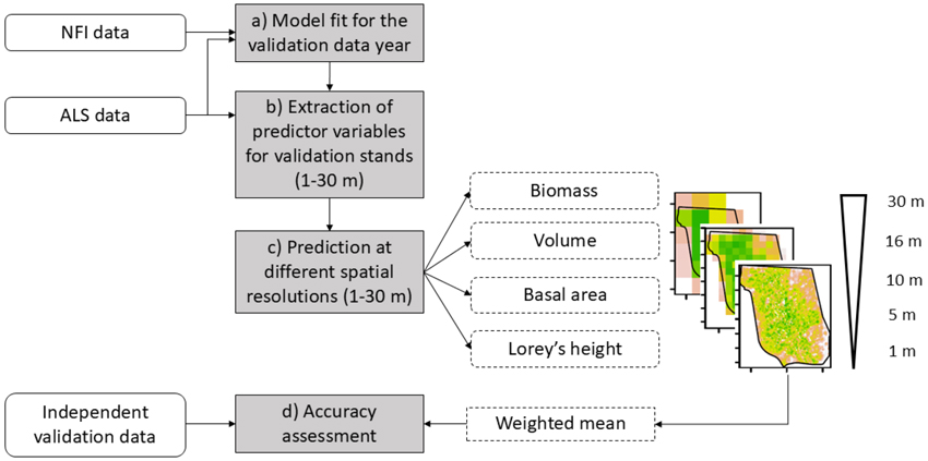
Fig. 2. Overview of the workflow used for assessing the uncertainty of Norwegian forest attribute models predicted at different spatial scales resolutions (1–30 m). The input datasets are indicated with rounded rectangles, the main steps (corresponding to a–d in the main text) are in grey rectangles, and intermediate data and processing steps are indicated with dashed rectangles respectively.
In step a), models for each measurement year of the validation data (2018, 2020, 2021, and 2022) were fitted (Fig. 2a) to match the validation field measurement date. This has been achieved by forecasting and backcasting the observed increments at the NFI plots to the field observation date of the validation stands. For example, if a validation stand was measured in 2022 and the NFI plots were measured between 2018 and 2022, we forecast the NFI plot values measured between 2018 and 2021 to 2022. In this way, inconsistency between the prediction date and the validation field measurement date was avoided. The predictor variables and regression models are described in sections 2.2.2 and 2.2.3.
In step b), we processed the ALS data at 1, 5, 10, 16, and 30 m spatial resolutions (Fig. 2b) for the validation stands (Fig. 1). We selected the ALS projects that were acquired closest in time to the field measurement date. The predictor variables were calculated for modeling biomass, volume, basal area, and Lorey’s height (the specific metrics are described in Section 2.2.2.). We calculated the time difference between the ALS acquisition date and the validation field measurement date, expressed as the number of growing seasons. Additionally, we resampled the dominant tree species (Breidenbach et al. 2021) and slope rasters from 16 m × 16 m resolution to the tested resolutions using nearest neighbor and bilinear interpolation. Information related to the ALS project and the geographic region was also added for the modeling process. The resampled slope raster was used as a predictor variable, the ALS project and geographic information as random effects and the dominant tree species map for stratification.
In step c), we applied the species-specific regression models – fitted at 16 m resolution – to predict biomass, volume, basal area, and Lorey’s height at the different spatial resolutions (1–30 m) for the pixels covering the validation stands (Fig. 2c). We then estimated forest attributes for pixels within the validation stands by calculating the mean of the predicted forest attributes at stand-level (Fig. 2d). Pixel predictions were weighted according to the proportion by which they covered the plots to account for the fact that not all pixels fully fall within them. To assess the accuracies at the stand level, the field plots measured within the validation stands (Fig. 1) have been aggregated using the mean of the predicted plot values. This process resulted in a dataset with (synthetic) estimates of forest attributes as predicted for the different pixel sizes which were used in the uncertainty assessment.
In step d), the uncertainty was evaluated by calculating the weighted root mean squared error (RMSE) and the weighted bias, taking into consideration the varying area sizes of the validation stands by:

with φ = 2 and ω = 0.5 for RMSE and φ = 1 and ω = 1 for bias, where![]() and
and![]() represent the observed and estimated forest attributes at stand level, and wi is the area of each validation stand; i = 1,…,n with n = 65 indices the validation stands. The relative RMSE and bias were calculated by dividing RMSE and bias by the mean of the observed values and multiplying the result by 100. Based on the dominant species at stand level, we also calculated the RMSE and bias per species group.
represent the observed and estimated forest attributes at stand level, and wi is the area of each validation stand; i = 1,…,n with n = 65 indices the validation stands. The relative RMSE and bias were calculated by dividing RMSE and bias by the mean of the observed values and multiplying the result by 100. Based on the dominant species at stand level, we also calculated the RMSE and bias per species group.
3 Results
In the stand-level validation of the Norwegian forest attribute map at its native resolution (16 m), the RMSEs were found to be 15.21%, 13.93%, 11.97%, and 6.87% for biomass, volume, basal area, and Lorey’s height, respectively (Table 2). The bias indicated an underestimation of ≤4.42% for biomass, volume and, Lorey’s height, and a slight overestimation for basal area (–0.10%) (Fig. 3, Table 2). Especially spruce-dominated stands with high biomass and volume tended to be underestimated (Figs. 3a,b). The RMSEs for basal area changed the least when changing the resolution and the lowest RMSE was observed at the native resolution. For the other attributes, the lowest RMSE was not observed at the native resolution (16 m) but at 5 m (biomass and volume) and 10 m (Lorey’s height) resolution (Table 2). The RMSEs across 1–30 m spatial resolutions (Table 2) showed a similar pattern for all attributes as they were highest for 1 m and 30 m, and decreased towards the pixel size with the lowest RMSE (Figs. 4a–d). The RMSEs ranged from 13.86% to 19.53% for biomass, 12.64% to 18.58% for volume. For Lorey’s height, the RMSE decreased with increasing spatial resolutions from 1 m to the native resolution (16 m) and increased slightly at 30 m resolution (Figs. 4e–h). Overall, the RMSE changes are relatively small (<5.95%) for the three additive attributes. For Lorey’s height as a non-additive attribute, the changes in RMSE were higher (18.41%).
| Table 2. Stand-level RMSE and bias for biomass, volume, basal area, and Lorey’s height, given predictions at different spatial resolutions for independent validation stands. The results for deciduous stands are derived from a limited number of observations (n = 4) and are provided solely for the sake of completeness. | |||||||||
| All species, n = 65 | |||||||||
| Biomass | Volume | Basal area | Lorey’s height | ||||||
| RMSE | bias | RMSE | bias | RMSE | bias | RMSE | bias | ||
| [%] | [%] | [%] | [%] | [%] | [%] | [%] | [%] | ||
| Resolution | 1 | 14.99 | –4.34 | 13.61 | –2.92 | 12.55 | –1.15 | 25.27 | –24.05 |
| 5 | 13.86 | –2.89 | 12.64 | –1.61 | 12.08 | 0.99 | 9.08 | –7.46 | |
| 10 | 14.17 | –3.63 | 12.96 | –2.46 | 11.99 | 0.73 | 6.86 | –3.87 | |
| 16 | 15.21 | –4.42 | 13.93 | –3.41 | 11.97 | 0.10 | 6.87 | –2.38 | |
| 30 | 19.53 | –7.79 | 18.58 | –6.98 | 13.20 | –2.52 | 7.38 | –1.54 | |
| Spruce, n = 30 | |||||||||
| Resolution | 1 | 14.32 | –8.28 | 13.45 | –7.21 | 11.13 | –1.52 | 25.97 | –24.87 |
| 5 | 12.31 | –5.87 | 11.92 | –4.97 | 10.19 | 1.59 | 9.61 | –8.33 | |
| 10 | 12.78 | –6.08 | 12.54 | –5.36 | 10.09 | 1.79 | 6.88 | –4.22 | |
| 16 | 13.81 | –6.61 | 13.47 | –6.01 | 9.98 | 1.50 | 6.91 | –2.45 | |
| 30 | 19.67 | –10.32 | 19.76 | –10.16 | 12.18 | –1.52 | 7.20 | –1.62 | |
| Pine, n = 31 | |||||||||
| Resolution | 1 | 12.88 | 1.79 | 12.49 | 1.99 | 13.39 | –0.77 | 25.72 | –24.8 |
| 5 | 13.45 | 1.82 | 12.27 | 1.97 | 13.13 | 0.35 | 8.61 | –7.18 | |
| 10 | 13.63 | 0.25 | 12.40 | 0.42 | 13.31 | –0.44 | 6.70 | –3.89 | |
| 16 | 14.42 | –0.99 | 13.12 | –0.97 | 12.99 | –1.39 | 6.59 | –2.68 | |
| 30 | 15.65 | –3.98 | 14.67 | –4.14 | 13.67 | –3.74 | 7.40 | –1.86 | |
| Broadleaf, n = 4 | |||||||||
| Resolution | 1 | 18.01 | –4.39 | 13.16 | 4.78 | 16.28 | –0.84 | 14.35 | –12.87 |
| 5 | 18.74 | –3.53 | 14.71 | 5.63 | 17.41 | 0.47 | 7.31 | –3.18 | |
| 10 | 18.45 | –4.38 | 13.27 | 4.93 | 16.31 | 0.19 | 7.14 | –1.26 | |
| 16 | 19.88 | –5.1 | 15.08 | 3.86 | 17.82 | –0.77 | 7.66 | 0.23 | |
| 30 | 19.79 | –7.99 | 12.49 | 2.74 | 16.13 | –2.09 | 8.01 | 1.32 | |
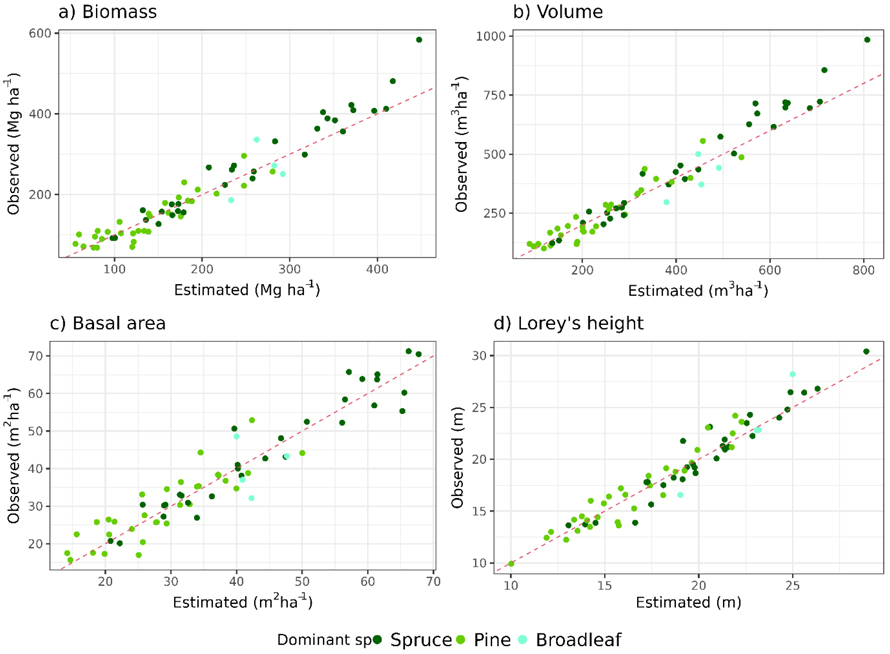
Fig. 3. Observed (field-based) versus estimated (lidar-based) values at the native resolution of the Norwegian forest attribute map at 16 m pixel size for each examined forest attribute (a: biomass, b: volume, c: basal area and d: Lorey’s height). The color of the dots indicates the dominant tree species within the validation stands.
The changes in bias across varying spatial resolutions showed a similar pattern as the RMSE. Overall, the smallest bias was observed at a 5 m resolution for biomass, volume, and at the native resolution for basal area. As an exception, the lowest bias for Lorey’s height was at 30 m resolution. The bias of biomass, volume, and basal area decreased from 1 m to 5 m, followed by an increasing trend up to 30 m resolution (Table 2, Figs. 4a–d). In contrast, the bias of Lorey’s height decreased from 1 m to 30 m (Table 2, Figs. 4g–h). While the differences in bias for biomass, volume , and basal area were relatively small (<5.37%), Lorey’s height had larger changes (22.51%).
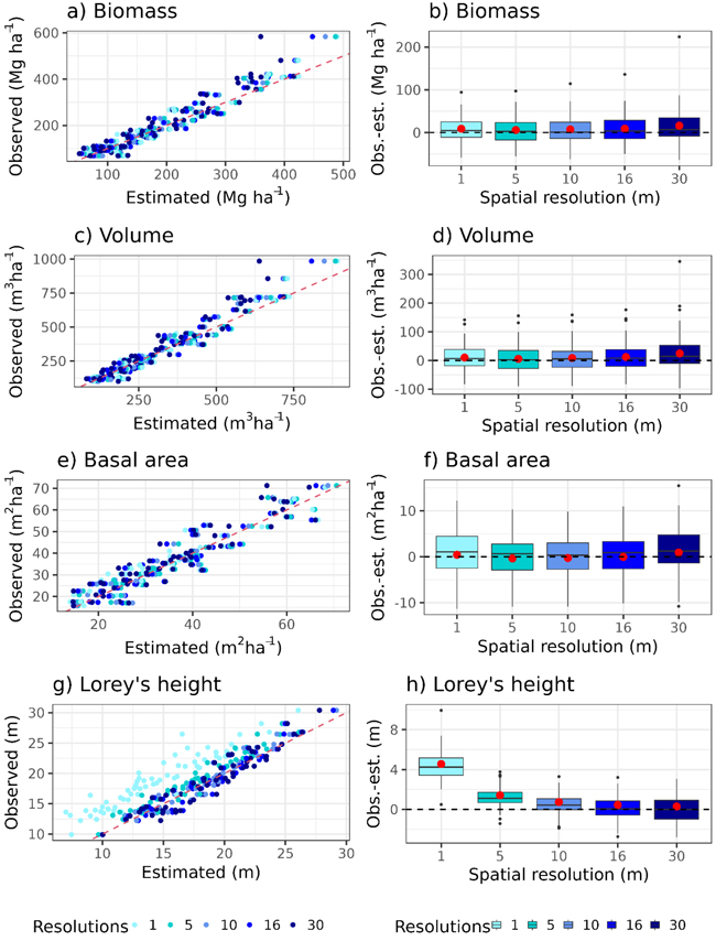
Fig. 4. Right column: Observed (field-based) versus estimated (lidar-based) values across different spatial resolutions for each forest attribute (a: biomass, c: volume, e: basal area, g: Lorey’s height). Left column: Corresponding boxplots illustrate the distribution of the difference between observed and estimated values at each spatial resolution and forest attributes (b: biomass, d: volume, f: basal area, h: Lorey’s height). The red dots indicate the area-weighted mean value of the difference between observed and estimated values.
We observe similar trends across spatial resolutions when comparing RMSE and bias of dominant species to the results for all species (Table 2). For spruce stands, RMSE values range from 6.88% to 25.97% and bias values range from –24.87 to 1.79% , which aligned with the results for all species. For pine stands, the RMSE values ranged from 6.59% to 25.72% and bias values ranged from –24.8% to 1.99% across all forest attributes, comparable with the results for all species. However, the lowest RMSE for volume are observed at 5 m resolution. Because broadleaf stands consist of only four observations, they are included in Table 2 solely for completeness.
4 Discussion
We evaluated the RMSE and bias of forest attribute maps (biomass, volume, basal area, and Lorey’s height) that were based on models fitted at a nominal resolution of 16 m which were used to predict maps with spatial resolutions ranging from 1 to 30 m. Except for Lorey’s height, the models use resolution-independent explanatory variables. The resulting estimates on stand level were compared to independent validation data at stand level.
The independent validation of the Norwegian forest attribute map at its native resolution showed lower RMSE and bias compared to previous studies. The RMSE values reported in this study are smaller by 5 to 21% compared to those of the cross-validation result of the Norwegian forest attribute map (Hauglin et al. 2021) and an independent validation conducted with forest management inventories (de Lera Garrido et al. 2023). The bias values in our study are in line with mean difference (MD) values reported by de Lera Garrido et al. (2023) , where independent field validation has been used. However, different approaches have been used to evaluate the uncertainty of the predicted forest attributes. Hauglin et al. (2021) assessed the predictions at the plot level where the uncertainties are larger, and de Lera Garrido evaluated the predictions by back casting the forest attributes maps to agree with the FMI field observation dates. The overall accuracies of volume, basal area, and Lorey’s height in our study are comparable with those reported in the Swedish forest attribute map by Nilsson et al. (2017).
The stand-level estimation of biomass, volume, and Lorey’s height in our study showed that the lowest RMSEs were not achieved at the native resolution, but at a 5 or 10 m resolution. As suggested by Packalen et al. (2019), this may be attributed to the fact that metrics derived from larger plots tend to yield regression coefficients that more accurately represent the true values at a finer spatial resolution. For basal area, we found that the highest accuracy was achieved at the native resolution, however, the difference in RMSE at 5 and 10 m resolution was less than 1%. Our findings regarding the trends in changes in RMSE at different spatial resolutions are in agreement with those from Packalen et al. (2019), who reported a slight decrease in RMSE for both resolution dependent and independent linear models for biomass at a finer spatial resolution (–0.05% to –0.34%) and a slight increase in RMSE at a coarser spatial resolution (up to 0.15%). We found this trend also applicable for volume, while it was only partly applicable for basal area and Lorey’s height. These two forest attributes show increased RMSE at 5 and 1 m resolutions. Nilsson et al. (2017) reported a small decrease in RMSE in the case of predicting volume and Lorey’s height at finer resolution in northern Sweden (changes in RMSE are 0.4% and 0.1%, respectively), which is in agreement with our findings. They, however, also reported a slight increase in RMSE for volume in Southern Sweden (2.1%) and for Lorey’s height (0.1%). Fassnacht et al. (2018) used simulated remote sensing data and observed small changes in RMSE and slightly decreased RMSE with increased plot size, which agrees with our findings. We also examined the RMSE trends with changing spatial resolutions according to the dominant species. The results suggest that comparable RMSE values achieved across all forest attributes and trends as observed in the aggregated results (Table 2).
We observe a slight underestimation for all attributes at the native resolution which is likely due to the fact that we used completely independent field validation data following slightly different measurement approaches and dates compared to the modelling data. Nonetheless, for the models with resolution-independent variables (biomass, volume, and basal area) for spatial resolutions of 5–30 m, we see the same trend as reported by Packalen et al. (2019) for biomass. The bias decreases when decreasing the pixel size relative to the native resolution and increases when increasing the pixel size relative to the native resolution. However, we also observed an increasing trend of the bias again at the finest resolution of 1 m. The dominant species-specific changes in bias across varying spatial resolutions overall showed the same trends compared to the aggregated results, just starting at different levels for the native resolution. Overall, it is a well-known issue that model-predicted maps based on remote sensing and empirical models result in biased estimates when aggregated (Breidenbach et al. 2022; Ståhl et al. 2024). However, unbiasedness is not a strict requirement at stand level as long as biases are not too large. It has also been shown that maps with large bias can be used to improve estimates if sufficient reference data are available (Räty et al. 2023).
We found that changes in RMSE and bias for the additive forest attributes to estimate at stand-level are small, a finding that is consistent with the results of Packalen et al. (2019). They reported that using resolution-independent predictor variables in the case of additive forest attributes such as biomass, a 4-times difference in resolution had a negligible effect on the uncertainty. We have further found that this result can be expanded for other additive forest attributes such as volume and basal area, and even a 16-times difference in resolution does not substantially affect the stand-level uncertainty. However, it needs to be noted that calculating the predictor variables (hmean_first, hmean_first_sq, h95_first, and prop_ab2m_first) at different spatial resolutions can capture different physical meanings, especially at 1 m resolution. For instance, the mean height of the first returns, reflects the canopy structure – higher values indicate larger canopy sizes and densities – at a 16 m resolution. This metric is useful for predicting, inter alia, volume, as canopy structure serves as a strong proxy for volume estimation. However, at finer resolutions (e.g., 1 m), the mean height of the first return may have a different interpretation, as individual pixels may not contain a single tree stem and should thus be zero which will not be the case when covering parts of the canopy . Even though some lidar metrics such as mean height allow for some physical interpretation, this is much less obvious for percentiles or metrics describing higher moments of the ALS distribution. Overall, our study suggests that with certain limitations and cautions, even Lorey’s height can be predicted at a different resolution than the NFI plot size as long as the resolution difference is less than 2 times compared to the native resolution. This finding aligns with Nilsson et al. (2017), who operationally used models for Lorey’s height fit at 25 m native resolution while predicting maps with 12.5 m resolution.
5 Conclusion
Growing accessibility of spatially explicit, nationwide forest attribute maps showcases their potential to provide wall-to-wall information about forest ecosystems, which can be used as a comprehensive knowledge base for various forest monitoring tasks. The required spatial resolution of these applications can deviate from the spatial resolution of map pixels given the reference plots. For instance, the proposed regulation on the European Forest Monitoring System allows countries to provide harmonized forest attribute maps at 10 m resolution, which typically will deviate the NFI plot sizes across the countries. Our results show that in an operational setting, the forest attribute models fitted at the NFI plot size can be used to predict finer spatial resolutions without large differences in RMSE and bias. Without the application of complex statistical scaling methods, the fitted model at the NFI plot size can be used to produce forest attribute maps at a 10 or 5 m spatial resolution that even resulted in slightly improved estimates on stand level. Even for extreme resolutions such as 1 m pixel size, the area-based approach can result in acceptable accuracies for additive forest attributes such as biomass, volume, and basal area.
Acknowledgments
We would like to acknowledge Stig Støtvig and Pauline Müller for their support in compiling the long-term trial data. Furthermore, we acknowledge Dr. Johannes Ralph and Dr. Marius Hauglin for providing advice and scripts based on their previous research. This study received funding from the EU under GA101056907 (PathFinder).
Author contributions
ZK conducted all data analyses, managed the study, and wrote the first draft. JB conceived the study, supervised the work, wrote parts of the manuscript, and acquired funding. Both authors accept the final version of the manuscript.
References
Astrup R, Rahlf J, Bjørkelo K, Debella-Gilo M, Gjertsen A-K, Breidenbach J (2019) Forest information at multiple scales: development, evaluation and application of the Norwegian forest resources map SR16. Scand J For Res 34: 484–496. https://doi.org/10.1080/02827581.2019.1588989.
Breidenbach J, Granhus A, Hylen G, Eriksen R, Astrup R (2020) A century of National Forest Inventory in Norway – informing past, present, and future decisions. For Ecosyst 7, article id 46. https://doi.org/10.1186/s40663-020-00261-0.
Breidenbach J, Waser LT, Debella-Gilo M, Schumacher J, Rahlf J, Hauglin M, Puliti S, Astrup R (2021) National mapping and estimation of forest area by dominant tree species using Sentinel-2 data. Can J For Res 51: 365–379. https://doi.org/10.1139/cjfr-2020-0170.
Breidenbach J, Ellison D, Petersson H, Korhonen KT, Henttonen HM, Wallerman J, Fridman J, Gobakken T, Astrup R, Næsset E (2022) Harvested area did not increase abruptly – how advancements in satellite-based mapping led to erroneous conclusions. Ann For Sci 79, article id 2. https://doi.org/10.1186/s13595-022-01120-4.
Dinerstein E, Vynne C, Sala E, Joshi AR, Fernando S, Lovejoy TE, Mayorga J, Olson D, Asner GP, Baillie JEM, Burgess ND, Burkart K, Noss RF, Zhang YP, Baccini A, Birch T, Hahn N, Joppa LN, Wikramanayake E (2019) A global deal for nature: guiding principles, milestones, and targets. Sci Adv 5, article id eaaw2869. https://doi.org/10.1126/sciadv.aaw2869.
Fassnacht FE, Latifi H, Hartig F (2018) Using synthetic data to evaluate the benefits of large field plots for forest biomass estimation with LiDAR. Remote Sens Environ 213: 115–128. https://doi.org/10.1016/j.rse.2018.05.007.
Fassnacht FE, White JC, Wulder MA, Næsset E (2023) Remote sensing in forestry: current challenges, considerations and directions. Forestry 97: 11–37. https://doi.org/10.1093/forestry/cpad024.
Geonorge (2024) Norge i bilder WMS-Ortophoto. https://register.geonorge.no/inspire-statusregister/norge-i-bilder-wms-ortofoto/dcee8bf4-fdf3-4433-a91b-209c7d9b0b0f. Accessed 29 October 2024.
Griscom BW, Adams J, Ellis PW, Houghton RA, Lomax G, Miteva DA, Schlesinger WH, Shoch D, Siikamäki JV, Smith P, Woodbury P, Zganjar C, Blackman A, Campari J, Conant RT, Delgado C, Elias P, Gopalakrishna T, Hamsik MR, Herrero M, Kiesecker J, Landis E, Laestadius L, Leavitt SM, Minnemeyer S, Polasky S, Potapov P, Putz FE, Sanderman J, Silvius M, Wollenberg E, Fargione J (2017) Natural climate solutions. Proc Natl Acad Sci USA 114: 11645–11650. https://doi.org/10.1073/pnas.1710465114.
Hauglin M, Rahlf J, Schumacher J, Astrup R, Breidenbach J (2021) Large scale mapping of forest attributes using heterogeneous sets of airborne laser scanning and National Forest Inventory data. For Ecosyst 8, article id 65. https://doi.org/10.1186/s40663-021-00338-4.
Hyyppä J, Hyyppä H, Leckie D, Gougeon F, Yu X, Maltamo M (2008) Review of methods of small-footprint airborne laser scanning for extracting forest inventory data in boreal forests. Int J Remote Sens 29: 1339–1366. https://doi.org/10.1080/01431160701736489.
Kangas A, Astrup R, Breidenbach J, Fridman J, Gobakken T, Korhonen KT, Maltamo M, Nilsson M, Nord-Larsen T, Næsset E, Olsson H (2018) Remote sensing and forest inventories in Nordic countries – roadmap for the future. Scand J For Res 33: 397–412. https://doi.org/10.1080/02827581.2017.1416666.
Köhl M, Magnussen SS, Marchetti M (2006) Sampling methods, remote sensing and GIS multiresource forest inventory. Springer Science & Business Media. https://doi.org/10.1007/978-3-540-32572-7.
de Lera Garrido A, Gobakken T, Hauglin M, Næsset E, Bollandsås OM (2023) Accuracy assessment of the nationwide forest attribute map of Norway constructed by using airborne laser scanning data and field data from the national forest inventory. Scand J For Res 38: 9–22. https://doi.org/10.1080/02827581.2023.2184488.
Magnussen S, Mandallaz D, Lanz A, Ginzler C, Næsset E, Gobakken T (2016) Scale effects in survey estimates of proportions and quantiles of per unit area attributes. Forest Ecol Manag 364: 122–129. https://doi.org/10.1016/j.foreco.2016.01.013.
Maltamo M, Næsset E, Vauhkonen J (eds) (2014) Forestry applications of Airborne Laser Scanning: concepts and case studies. Springer, Dordrecht, Netherlands. https://doi.org/10.1007/978-94-017-8663-8.
Maltamo M, Packalen P, Kangas A (2021) From comprehensive field inventories to remotely sensed wall-to-wall stand attribute data – a brief history of management inventories in the Nordic countries. Can J For Res 51: 257–266. https://doi.org/10.1139/cjfr-2020-0322.
McRoberts RE, Tomppo EO, Næsset E (2010) Advances and emerging issues in national forest inventories. Scand J For Res 25: 368–381. https://doi.org/10.1080/02827581.2010.496739.
Næsset E (2002) Predicting forest stand characteristics with airborne scanning laser using a practical two-stage procedure and field data. Remote Sens Environ 80: 88–99. https://doi.org/10.1016/S0034-4257(01)00290-5.
Næsset E (2014) Area-based inventory in Norway – from innovation to an operational reality. In: Maltamo M, Næsset E, Vauhkonen J (eds) Forestry applications of Airborne Laser Scanning: concepts and case studies. Springer, Dordrecht, Netherlands, pp 215–240. https://doi.org/10.1007/978-94-017-8663-8_11.
Næsset E, Gobakken T, Holmgren J, Hyyppä H, Hyyppä J, Maltamo M, Nilsson M, Olsson H, Persson Å, Söderman U (2004) Laser scanning of forest resources: the nordic experience. Scand J For Res 19: 482–499. https://doi.org/10.1080/02827580410019553.
NIBIO (2024) Kilden. https://kilden.nibio.no/. Accessed 29 October 2024.
Nilsson M, Nordkvist K, Jonzén J, Lindgren N, Axensten P, Wallerman J, Egberth M, Larsson S, Nilsson L, Eriksson J, Olsson H (2017) A nationwide forest attribute map of Sweden predicted using airborne laser scanning data and field data from the National Forest Inventory. Remote Sens Environ 194: 447–454. https://doi.org/10.1016/j.rse.2016.10.022.
Nord-Larsen T, Schumacher J (2012) Estimation of forest resources from a country wide laser scanning survey and national forest inventory data. Remote Sens Environ 119: 148–157. https://doi.org/10.1016/j.rse.2011.12.022.
Packalen P, Strunk J, Packalen T, Maltamo M, Mehtätalo L (2019) Resolution dependence in an area-based approach to forest inventory with airborne laser scanning. Remote Sens Environ 224: 192–201. https://doi.org/10.1016/j.rse.2019.01.022.
Pinheiro J, Bates D (2000) Mixed-effects models in S and S-PLUS. Springer Science & Business Media. https://doi.org/10.1007/b98882.
Rahlf J, Hauglin M, Astrup R, Breidenbach J (2021) Timber volume estimation based on airborne laser scanning – comparing the use of national forest inventory and forest management inventory data. Ann For Sci 78, article id 49. https://doi.org/10.1007/s13595-021-01061-4.
Räty J, Hauglin M, Astrup R, Breidenbach J (2023) Assessing and mitigating systematic errors in forest attribute maps utilizing harvester and airborne laser scanning data. Can J For Res 53: 284–301. https://doi.org/10.1139/cjfr-2022-0053.
Ståhl G, Gobakken T, Saarela S, Persson HJ, Ekström M, Healey SP, Yang Z, Holmgren J, Lindberg E, Nyström K, Papucci E, Ulvdal P, Ørka HO, Næsset E, Hou Z, Olsson H, McRoberts RE (2024) Why ecosystem characteristics predicted from remotely sensed data are unbiased and biased at the same time – and how this affects applications. For Ecosyst 11, article id 100164. https://doi.org/10.1016/j.fecs.2023.100164.
Thompson I, Mackey B, McNulty S, Mosseler A (2009) Forest resilience, biodiversity, and climate change. A synthesis of the biodiversity/resilience/stability relationship in forest ecosystems. Technical Series 43, Secretariat of the Convention on Biological Diversity, Montreal. ISBN 92-9225-137-6.
Tomppo E, Haakana M, Katila M, Peräsaari J (2008) Multi-Source National Forest Inventory – methods and applications. Managing Forest Ecosystems 18, Springer. ISBN 978-1-4020-8712-7.
Tuominen S, Pitkänen T, Balazs A, Kangas A (2017) Improving Finnish Multi-Source National Forest Inventory by 3D aerial imaging. Silva Fennica 51, article id 7743. https://doi.org/10.14214/sf.7743.
Total of 32 references.
