Jonas R. Coussement,
Kathy Steppe,
Peter Lootens,
Isabel Roldán-Ruiz,
Tom De Swaef 
A flexible geometric model for leaf shape descriptions with high accuracy
Coussement J. R., Steppe K., Lootens P., Roldán-Ruiz I., De Swaef T. (2018). A flexible geometric model for leaf shape descriptions with high accuracy. Silva Fennica vol. 52 no. 2 article id 7740. https://doi.org/10.14214/sf.7740
Highlights
- A method for assessing leaf shape for 3D plant models is proposed
- The model is highly flexible and fits a large variety of shapes
- It allows analysis of shape differences within and between leaf datasets.
Abstract
Accurate assessment of canopy structure is crucial in studying plant-environment interactions. The advancement of functional-structural plant models (FSPM), which incorporate the 3D structure of individual plants, increases the need for a method for accurate mathematical descriptions of leaf shape. A model was developed as an improvement of an existing leaf shape algorithm to describe a large variety of leaf shapes. Modelling accuracy was evaluated using a spatial segmentation method and shape differences were assessed using principal component analysis (PCA) on the optimised parameters. Furthermore, a method is presented to calculate the mean shape of a dataset, intended for obtaining a representative shape for modelling purposes. The presented model is able to accurately capture a large range of single, entire leaf shapes. PCA illustrated the interpretability of the parameter values and allowed evaluation of shape differences. The model parameters allow straightforward digital reconstruction of leaf shapes for modelling purposes such as FSPMs.
Keywords
image processing;
leaf contour;
leaf shape;
shape function;
digitising;
tree leaf shape
- Coussement, Plant Sciences Unit, Institute for Agricultural and Fisheries Research (ILVO), Caritasstraat 39, B-9090 Melle, Belgium; Laboratory of Plant Ecology, Department of Plants and Crops, Faculty of Bioscience Engineering, Ghent University, Coupure links 653, B-9000 Ghent, Belgium E-mail jonas.coussement@ilvo.vlaanderen.be
- Steppe, Laboratory of Plant Ecology, Department of Plants and Crops, Faculty of Bioscience Engineering, Ghent University, Coupure links 653, B-9000 Ghent, Belgium E-mail kathy.steppe@ugent.be
- Lootens, Plant Sciences Unit, Institute for Agricultural and Fisheries Research (ILVO), Caritasstraat 39, B-9090 Melle, Belgium E-mail peter.lootens@ilvo.vlaanderen.be
- Roldán-Ruiz, Plant Sciences Unit, Institute for Agricultural and Fisheries Research (ILVO), Caritasstraat 39, B-9090 Melle, Belgium; Department of Plant Biotechnology and Bioinformatics, Faculty of Sciences, Ghent University, Technologiepark Zwijnaarde 927, B-9052 Zwijnaarde, Belgium E-mail isabel.roldan-ruiz@ilvo.vlaanderen.be
-
De Swaef,
Plant Sciences Unit, Institute for Agricultural and Fisheries Research (ILVO), Caritasstraat 39, B-9090 Melle, Belgium
E-mail
tom.deswaef@ilvo.vlaanderen.be
Received 1 June 2017 Accepted 23 February 2018 Published 1 March 2018
Views 65289
Available at https://doi.org/10.14214/sf.7740 | Download PDF

Supplementary Files
1 Introduction
The shape of plant leaves plays an important role in various fields of study. Their diagnostic value is important in the field of systematics, where the taxonomy of closely related species, natural hybrids or subspecies is studied (Jensen et al. 2002), and paleobotany, where leaf geometry is used as proxy for paleoclimatic and paleoecological variables (Royer et al. 2005). In agricultural engineering, leaf shape analysis is essential for automated species recognition, which has applications in site-specific weed control and herbicide application using machine vision or remote sensing (Meyer 2011). Similarly, in forest ecosystem monitoring, the ability to capture and model the structural complexity of the forest canopy is one of the main constraints in method development and can lead to inconsistencies when neglected (Côté et al. 2011). In the fields of plant modelling and ecophysiology, accurate descriptions of the leaves’ spatial arrangement and shape play a crucial role in the study of a plant’s interaction with its environment. The structure of the forest or crop canopy, which is the combination of leaf shape, size and spatial orientation, constitutes the major interface between the plant and its aerial environment, and thus influences important ecophysological factors such as boundary layer resistance and radiation interception, which heavily impact the fluxes of water, heat and carbon (Prusinkiewicz et al. 1994). The prediction of these complex interactions and how morphological traits influence the final production is an important issue for applications such as plant breeding (Bergez et al. 2013). This makes a mathematical description and simulation of realistic leaf shapes indispensable in plant and tree models that take 3D geometry into account, such as functional-structural plant models (FSPMs) (Perttunen et al. 1996; Henke et al. 2014).
The purpose of geometric leaf descriptors is to provide a set of landmarks or parameters for a model, which allow the unambiguous approximation or identification of a leaf shape based on collected data. The level of geometrical detail contained in these descriptors depends on the application. A complex model may consist of large sets of parameters, which allow for a detailed and unbiased description of the leaf shape. Such descriptors can be useful in species determination, where the large set of parameters can be analysed through means of principal component or discriminant analysis (Neto et al. 2006), or for rendering realistic 3D scenes. A less complex model can provide a simplified though accurate representation of the leaf shape suitable for modelling purposes by saving substantial computation time (Fournier and Pradal 2012).
The most straightforward way to describe a leaf shape is by approximating the leaf width as a function of the distance to the leaf base by curve-fitting. This can be achieved using polynomials (Fournier et al. 2003), smoothing splines (Mündermann et al. 2005; Henke et al. 2014) or hermit curves (Henke et al. 2014). These methods are able to accurately describe simple leaf shapes, but have non-functional parameters, and therefore, cannot be directly interpreted as geometric features. Consequently, two morphologically very similar leaves can yield distinctly different parameter sets limiting applications such as studying leaf growth, as a small change in leaf shape during growth will not be captured by the gradual progression of one or a few parameters, but by a change of the entire parameter set. This limitation can be overcome by adapting the polynomial functions to contain only functional parameters such as curvature parameters (Dornbusch et al. 2007; Evers et al. 2007). While this works well for the lanceolate leaves of Gramineae, these functions are unable to capture more complex shapes (e.g. cordate leaves) due to their inherent inability to describe multivalued function shapes.
Another way to obtain geometric descriptors of leaf shape is by contour-fitting techniques, of which elliptic Fourier analysis (Iwata et al. 2002; Neto et al. 2006) allows near-perfect description of the leaf contour. However, the accuracy of this approach depends on the number of harmonics (h) used, resulting in 4h – 3 parameters. A typical approximation uses the first 20 (Iwata et al. 2002) or 30 (Neto et al. 2006) harmonics resulting in 77 or 117 (non-functional) parameters, respectively. While this imposes no limitations for multivariate analysis, such a number of parameters are not practically applicable for plant and tree models (Henke et al. 2014). Bézier curves (Chi et al. 2003) allow the description of a multivalued function with a low number of functional parameters. These are ideal for describing the general shape of plant leaves for applications such as species identification and growth measurements, but lack the flexibility to accurately describe more complex shapes.
Ideally, a leaf shape model should be applicable to a wide variety of leaf shapes and strive for an optimum between complexity and accuracy with parameters that are geometrically interpretable (i.e. functional). To this end, Young (2010) presented a simple shape algorithm that is capable of generating a large variety of leaf shapes with a small number of parameters. The starting condition of the algorithm is a line of points, representing the midrib of the leaf. These points are assigned a growth rate and growth direction using the model parameters and their relative position on the midrib. In each step of the algorithm, these points grow outward, following their assigned direction and growth rate, causing an exponential growth pattern. These “growth” parameters apply to the progression of the algorithm, and have no biological interpretation (i.e. they do not represent the growth of the leaf). Young’s primary focus was to capture the range of biological diversity in leaf shapes with a general and conceptually simple algorithm rather than accurately describing individual leaves. Therefore, the algorithm was kept relatively simple and has certain limitations in terms of flexibility and geometrical interpretability of the parameters.
This paper presents an adjustment to Young’s algorithm to resolve the limitations on parameter interpretability and flexibility. More specifically, the abstract “growth” concept was discarded, and the concepts of direction and length (i.e. “growth” rate) were modified into more flexible functions to enable description of a large variety of single, entire leaf shapes. The model was applied to leaf scan data of a variety of leaf shapes (from seven tree species) to illustrate the model accuracy and the diagnostic interpretability of the model parameters. Furthermore, a method is described to allow calculation of the mean leaf shape in a dataset.
2 Materials and methods
2.1 Data acquisition
Seven tree species were selected from an existing leaf dataset (Mallah et al. 2013) based on their large shape differences to acquire a wide range of single leaf shapes. While this sample contains only trees, we believe the diversity of shapes to be sufficient to illustrate the applicability of the shape model for other plant species. The selection contained mask images for 16 different leaves derived from Alnus cordata (Loisel.) Duby, Arundinaria simonii (Carrière) Rivière & C. Rivière, Cercis siliquastrum L., Cercis siliquastrum F.Buerger ex Hance var. Chinensis, Argyrocytisus battandieri (Maire) Raynaud, Ginkgo biloba L. and Tilia oliveri Szyszył. These mask images were manually manipulated to remove the leaf petiole (if present) and to align the central vein of each leaf with the x-axis using the image manipulation software GIMP. Afterwards, contour coordinates were extracted by automated processing of the resulting images using the Python component of OpenCV. Finally, the contours were split at the midrib and normalised (i.e. length of midrib and width of the half leaf were set to one). Leaf model implementation, parameter optimisation, principal component analysis (PCA) and mean leaf shape calculation were carried out in RStudio.
2.2 Leaf shape model
The model describes the outline of a half leaf by progression of an internal variable j (0 ≤ j ≤ 1)describing the position (j,0) on the leaf midrib. Each value of j corresponds to a coordinate on the leaf edge (xj,yj) (Fig. 1). This transformation is represented by a vector, of which the length and the orientation are determined by the value of j. The length of this vector is described by gL (0 ≤ gL ≤ 1), with its progression depending on the complexity of the leaf shape. In any case, the point at the leaf base and leaf tip correspond to the same point on the leaf edge, namely (0,0) and (1,0). Therefore, the length gL of their transformation vector is zero. For the common entire shape of many leaves, a single point jd can be located where the width is maximal (i.e. gL = 1), with gL strictly increasing from the leaf base to jd and strictly decreasing to the leaf tip. A simple power law dependence is well-suited to describe such behaviour (Young 2010):
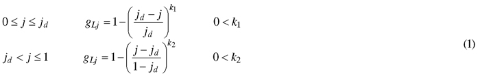
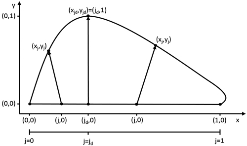
Fig. 1. The model describes the leaf outline through a transformation of every point (j,0) on the leaf midrib. The size and orientation of these transformation vectors are dependent on the value of j. At the point of maximal width jd, the size of the this vector is 1 and its slope 0.
The magnitude of exponents k1 and k2 determine the drop-off rate of gL towards the leaf base and tip, respectively (Fig. 2).
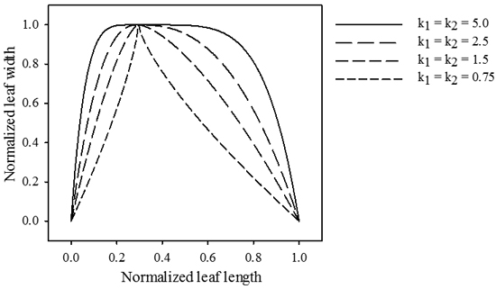
Fig. 2. Influence of parameters k1 and k2 on the relative length of the transformation vector across the leaf midrib. jd = 0.3, b1 = b2 = 0.
The orientation of the transformation vectors is described by a slope value s, which is equal to tangent of the angle between the transformation vector and the midrib normal. Consequently, s = 0represents a positive orientation parallel to the y-axis, a negative value for s represents a rotation to the left and a positive value a rotation to the right. In the simplest case, a constant value for s can be used (as done in Young (2010)). However, this limits model flexibility and hinders the interpretability of parameter jd, as it will no longer indicate the relative position of maximal width on the leaf midrib. Therefore, we assured the fixed position of the maximal leaf width by assigning a value of zero to the slope at jd. Coordinates closer to the leaf base get assigned a negative slope value and those closer to the leaf tip a positive slope value. Progression of these values in terms of j can be described by a variety of functions depending on the complexity of the leaf that is to be described. In the general case of entire shapes, another power law dependence can be used:
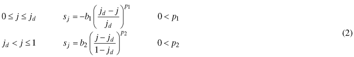
Contrasting to the functions describing the vector length, these functions achieve their maximal absolute value at the leaf base and tip. The magnitudes of b1 and b2 determine the maximal strength of the slope (Fig. 3), while p1 and p2 dictate the rate at which the slope increases (Fig. 4). Positive values for b1 and b2 cause the leaf to bulge outwards, negative values bulge inwards.
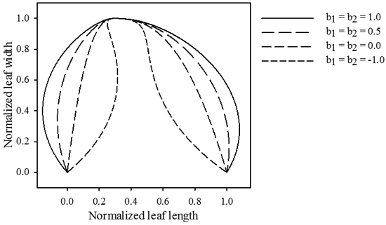
Fig. 3. Influence of parameters b1 and b2. The magnitude of these parameters determines the size of the formed extrusions. Positive values cause the leaf to push outwards, while negative values cause an inwards movement. jd = 0.3 , k1 = k2 = 2.5, p1 = p2 = 2.5.
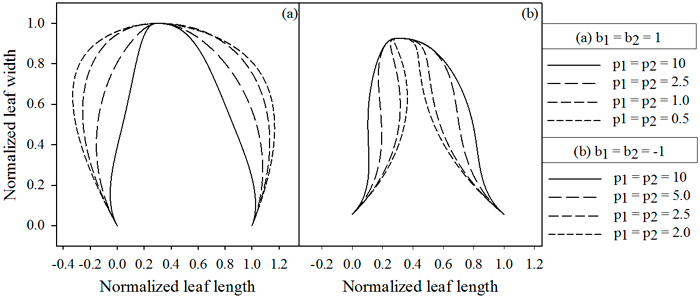
Fig. 4. Influence of parameters p1 and p2, which depend on the value of b. (A) b = 1, (B) b = –1. Lowering the parameter values cause the extrusions to move away from the midrib, while higher values cause them to move towards the midrib. jd = 0.3 , k1 = k2 = 2.5.
As the position of the coordinates changes according to the length and orientation of their transformation vectors, the change in coordinates from the leaf midrib to the leaf outline can be calculated using Pythagoras’ theorem:
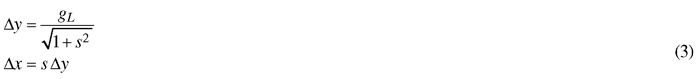
Therefore, the coordinates of the leaf edge are described by the following parametric equation:
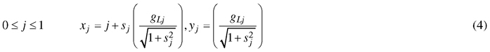
Concretely, these equations split each leaf side further into quadrants by the position of jd with parameters k1, b1, p1 and k2, b2, p2 describing the quadrants closest to the leaf base and tip, respectively.
2.3 Model performance evaluation
Model performance was evaluated by comparing the segmentation of an area containing the input leaf with the model description using R packages “sp” and “rgeos” (Bivand et al. 2013; Bivand and Rundel 2017). This resulted in four regions (Smochina 2011) (Fig. 5):
- True Positive (TP) areas contain leaf surface that are captured by the model description;
- False Positive (FP) areas contain no leaf surface, but are described as leaf by the model;
- True Negative (TN) areas contain no leaf surface and are not described as leaf by the model;
- False Negative (FN) areas contain leaf surface, but are not captured by the model.
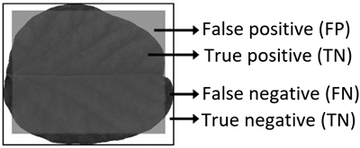
Fig. 5. Illustrative example of model performance criterion areas when a leaf is classified as a square.
As this definition does not specify the size of TN around the leaf, TN was redefined as:
![]()
These values were then used to calculate the accuracy (Acc) of the model (Smochina 2011):
![]()
which represents the portion of correctly classified area (both leaf and non-leaf) by the model.
2.4 Parameter optimisation
A parameter optimisation was conducted to find the optimal parameter sets that best described each individual leaf half according to the accuracy criterion (Eq. 6). Due to the multi-dimensionality of this problem with respect to model parameters, optimisation was done by applying a genetic algorithm to find the global minimum using R package “genalg” (Willighagen and Ballings 2015). A genetic algorithm is a constrained optimisation (i.e. the boundaries of each parameter must be set prior to optimisation), which allows i) the elimination of nonsensical parameter combinations (e.g. negative values for k1,2) and ii) maintaining the geometric interpretability jd as the position on which the leaf reaches its maximal width, while still allowing a broad search within the parameter space. Therefore, k1,2 was constrained between 0and 10, b1,2 between –10 and 10 and p1,2 between 0and 20. Parameter jd was set to allow a maximal deviation of 0.1 from the true relative position of maximal width in the data.
2.5 Mean leaf shape calculation
The mean leaf shape of each group cannot be calculated by simply averaging each parameter in the set due to the inherent interdependency of the parameters k, b and p in each quadrant of the leaf, i.e. the magnitude of these parameters heavily affects the contribution of the other parameters to the size and shape of each quadrant. Therefore, a set of comparable pseudo-landmarks (Dryden and Mardia 1998) needed to be defined on the outline of each (half) leaf.
This was achieved by calculating the intersections of a set of lines originating in the leaf centroid, defined as (jd,0), at an incrementing angle α with the leaf contour (Fig. 6). An arbitrary value of α = 2° was chosen, resulting in a set of 91 pseudo-landmarks. In Ginkgo, the centroid definition was shifted to (1,0) to ensure a single intersection for each line. The resulting coordinates serve as a set of pseudo-landmarks which can be averaged across the samples, resulting in a description of the mean leaf shape.
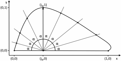
Fig. 6. Definition of pseudo-landmarks for calculating the mean leaf shape. α = ![]() with n + 1 the amount of pseudo-landmarks.
with n + 1 the amount of pseudo-landmarks.
3 Results
The flexibility of the model allows an accurate description of all selected single, entire leaf shapes (Fig. 7). On average, the model overestimated the normalised area of the leaves by 0.14%, and modelled them with an accuracy (as defined by Eq. 6) of 97.88%. The means and confidence intervals of the normalised area, and the accuracy of the model for each leaf group are given in Table 1.
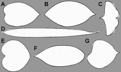
Fig. 7. Optimised model description (solid line) of a random leaf sample in all seven tree species (Mallah et al. 2013): Alnus cordata (A), Cornus kousa (B), Ginkgo biloba (C), Arundinaria simonii (D), Cercis siliquastrum (E), Argyrocytisus battandieri (F) and Tilia oliveri (G) plotted on the original data (white mask image).
| Table 1. Comparison of the normalised area of the leaves of the seven selected tree species with their respective model fits. The accuracy of the model fit as defined in Eq. 6 is also given for each species. | |||
| Species name | Area (Data) Mean – [95% CI] | Area (Fit) Mean – [95% CI] | Accuracy Mean – [95% CI] |
| Alnus cordata | 0.746 [0.710–0.800] | 0.748 [0.712–0.801] | 0.984 [0.980–0.987] |
| Arundinaria simonii | 0.719 [0.684–0.784] | 0.718 [0.683–0.779] | 0.978 [0.970–0.984] |
| Cercis siliquastrum | 0.934 [0.868–1.057] | 0.936 [0.871–1.053] | 0.982 [0.974–0.988] |
| Cornus kousa | 0.648 [0.623–0.688] | 0.646 [0.621–0.687] | 0.989 [0.986–0.992] |
| Argyrocytisus battandieri | 0.714 [0.692–0.731] | 0.711 [0.689–0.725] | 0.987 [0.983–0.991] |
| Ginkgo biloba | 0.735 [0.618–0.879] | 0.726 [0.614–0.864] | 0.956 [0.941–0.972] |
| Tilia oliveri | 0.749 [0.720–0.789] | 0.754 [0.724–0.794] | 0.976 [0.970–0.980] |
The interpretability of the parameters can be illustrated using a PCA on the parameter sets of the different plant species. For illustrative purposes, a PCA is shown for the half leaves of three distinctly different leaf types: i) the aristate shape of Cornus, ii) the reniform shape of Cercis and iii) the flabellate shape of Ginkgo (Fig. 8). It clearly shows how Ginkgo leaves distinguish themselves from Cornus and Cercis leaves by having relatively:
- Large values for k2 and b2, which indicates an outward bulge at the leaf tips,
- A large value for p2 indicating this bulge is oriented close to the leaf midrib,
- Low values for k1, b1, indicating an inward bulge at the leaf petiole.
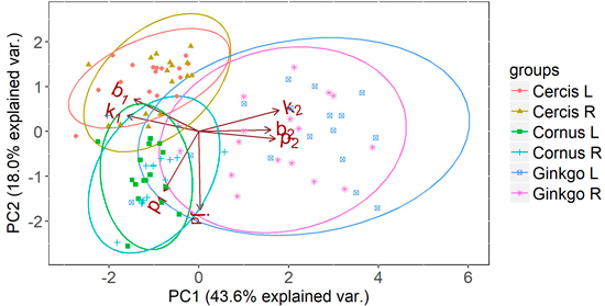
Fig. 8. Principal component analysis (PCA) on the parameters of the half leaf samples (where L and R represent the left and right side of the leaf respectively) of Cornus, Cercis and Ginkgo indicating the principal shape differences between groups expressed in relative difference in shape parameters. The ellipses represent the 95% confidence intervals for each group. Overlapping ellipses indicate similarity between groups, and point to symmetry in the leaves.
Similarly, Cercis is distinguished by high values for k1 and b1, combined with a low value for p1, illustrating the presence of an outward leaf bulge oriented away from the leaf midrib. Cornus is mainly distinguished by the high value for p1. Combined with moderate values for k1 and b1 this can indicate an acute leaf base. The low values of k2, b2, and p2 may suggest the presence of a leaf tip. It must be noted however, that the PCA plot shows relative rather than absolute parameter values. Therefore, PCA is a good tool to compare relative shape differences but direct interpretation of shape from the model parameters should preferably be done directly on the absolute model parameters.
The calculated mean leaf shapes underestimate the true mean area ranging from 0.13% in Alnus to 3.82% in Ginkgo (Table 2).
| Table 2. Comparison of the mean normalised area of the leaves of the seven selected tree species with the normalised area of the calculated mean leaf shape for each group. | |||
| Species name | Mean area (Data) | Area mean shape | Relative difference in area |
| Alnus cordata | 0.746 | 0.745 | –0.13% |
| Arundinaria simonii | 0.719 | 0.708 | –1.59% |
| Cercis siliquastrum | 0.934 | 0.931 | –0.35% |
| Cornus kousa | 0.648 | 0.641 | –1.15% |
| Argyrocytisus battandieri | 0.714 | 0.708 | –0.82% |
| Ginkgo biloba | 0.735 | 0.707 | –3.82% |
| Tilia oliveri | 0.749 | 0.742 | –0.93% |
4 Discussion
The model presented in this paper was built on the concepts of the growth-algorithm model presented by Young (2010) with the intention of improving flexibility and parameter interpretability to describe individual leaves with high accuracy. The notion of using an internal variable to describe the leaf outline through transformation vectors proved a useful approach to describe a large variety of leaves with the inclusion of a slope variable to deal with multivalued function shapes. However, Young’s algorithm relies on multiple evaluations of the model (i.e. the transformation vectors are applied several times) to generate leaf shapes. Hence, the number of evaluation steps determines the final size of the leaf, but also alters its shape. This method is not suited for dealing with normalised shapes and hinders evaluation of the contribution of each parameter to the leaf’s shape. Secondly, Young represents the slope of the transformation vectors as a constant. This results in a low flexibility of the model, but also hinders the interpretation of jd which then no longer corresponds to the point of maximal width. These problems were addressed to create an improved model, suited for mathematically describing the outlines of a large variety of single, entire leaf shapes.
In its current form, the shape of each leaf half is described by seven parameters (i.e. jd, k1, k2, b1, b2, p1 and p2), which results in a required 15 parameters for a full leaf shape description, including a single parameter describing the proportion of each leaf half to the entire normalised leaf. Additionally, the length and width of the leaf are required for a full digital reconstruction of the leaf on the original scale.
In applications where a low amount of parameters is preferred over high accuracy, a number of simplifications to the model can be made. Firstly, a PCA analysis can be used on the opposing leaf halves to assess whether the leaves can be assumed symmetrical (Fig. 8). If this is the case, the parameter set can be reduced from 15 to 7, as a proportionality parameter is then redundant. Secondly, in the case of very similar leaves (e.g. a single species), less flexibility is required. This allows the user to replace one or more parameters with well-chosen constants, effectively fine-tuning the model for the leaves in question.
In comparison to other methods, this model provides the advantage of being able to describe multivalued function shapes (as opposed to polynomials (Fournier et al. 2003), smoothing splines (Mündermann et al. 2005; Henke et al. 2014) or hermit curves (Henke et al. 2014)) with high flexibility (as opposed to Bézier curves (Chi et al. 2003)) and a relatively low amount of diagnostic parameters (as opposed to elliptic Fourier analysis (Iwata et al. 2002; Neto et al. 2006)).
Aside from the leaf shape model, a method was presented for calculating the mean leaf shape as a simplified version of the Procrustes mean shape (Stegmann and Gomez 2002). Where the presented mean shape is obtained by immediate comparison of the acquired landmarks, the Procrustes mean allows additional rotation and rescaling of the landmarks in order to optimise the shape alignment. These additional operations are redundant in this case as scaling was removed during normalisation, and the orientation is fixed due to the presence of the leaf petiole. The method for acquiring the landmarks was chosen to obtain a large, unambiguous set of comparable landmarks. The resulting mean shapes are good representations of the shapes in each group, demonstrated by their normalised area which closely approximates the true group mean (Table 2). The larger deviation of Ginkgo can be ascribed to a combination of large shape variability in the dataset and the irregular edges at the leaf tips.
Calculation of the mean leaf shape allows for the generation of a single representative shape of a leaf dataset. Combining this with an architectural model, results in a detailed description of the canopy. In the case of crop models, this allows straightforward evaluation of how leaf shape differences between plant genotypes influence crop characteristics such as light interception and photosynthesis for plant ideotyping (Sarlikioti et al. 2011). This presents a significant increase in model complexity to classical crop models, which often represent the crop canopy as a fixed nu mber of horizontal layers (e.g. comparison in Confalonieri et al. 2016). However, it can provide a solution to inconsistencies arising from neglecting canopy complexity such as leaf senescence resulting from self-shading and leaf age (Stella et al. 2014). Furthermore, proper simulation of tree light interception could be of major importance in understanding the microclimate, and thus growth conditions, of understorey plant species (De Frenne et al. 2013). Inclusion of such complexity substantially increases the performance of modelling light interception, but also allows simulation of the effect of individual leaves on tree hydraulics (de Reffye et al. 1997) and detailed descriptions of adaptation to light of individual leaves in the crown (Eschenbach 2000).
The presented model for capturing the planar leaf shape of trees can smoothly be extended for an even more detailed 3D leaf representation by including additional equations, which independently describe the progression of potential z-coordinates (Supplementary file S1: Fig. S.1). However, parameterisation of this additional complexity requires 3D digitising using in situ photographs from different perspectives or use of digitisers (Falster and Westoby 2003; Evers et al. 2005; Dornbusch et al. 2007; Dauzat et al. 2008), which was not the focus of our study.
In this paper a highly flexible and customisable model has been presented for the digitalisation of single, entire leaf shapes. The model was demonstrated for seven contrasting leaf shapes, illustrating the model’s capability of capturing a large range of shapes with high accuracy. The interpretability of the parameters allows evaluation of (dis)similarities between leaf groups or opposing leaf halves through PCA. The presented method for calculating the mean shape of a group offers perspectives for modelling purposes such as FSPMs.
Acknowledgements
This work was supported by an individual PhD grant issued by the Agency for Innovation by Science & Technology (IWT) to Jonas Coussement.
References
Bergez J.E., Chabrier P., Gary C., Jeuffroy M.H., Makowski D., Quesnel G., Ramat E., Raynal H., Rousse N., Wallach D., Debaeke P., Durand P., Duru M., Dury J., Faverdin P., Gascuel-Odoux C., Garcia F. (2013). An open platform to build, evaluate and simulate integrated models of farming and agro-ecosystems. Environmental Modelling and Software 39: 39–49. https://doi.org/10.1016/j.envsoft.2012.03.011.
Bivand J.E., Rundel C. (2017). rgeos: interface to geometry engine – open source (‘GEOS’). R package version 0.3-26. https://CRAN.R-project.org/package=rgeo.
Bivand R.S., Pebesma E., Gomez-Rubio V. (2013). Applied spatial data analysis with R. Second edition. Springer, NY. http://www.asdar-book.org/.
Chi Y.T., Chien C.F., Lin T.T. (2003). Leaf shape modeling and analysis using geometric descriptors derived from Bezier curves. Transactions of the ASAE 46(1): 175–185. https://doi.org/10.13031/2013.12540.
Confalonieri R., Orlando F., Paleari L., Stella T., Gilardelli C., Movedi E., Pagani V., Cappelli G., Vertemara A., Alberti L., Alberti P., Atanassiu S., Bonaiti M., Cappelletti G., Ceruti M., Confalonieri A., Corgatelli G., Corti P., Dell’Oro M., Ghidoni A., Lamarta A., Maghini A., Mambretti M., Manchia A., Massoni G., Mutti P., Pariani S., Pasini D., Pesenti A., Pizzamiglio G., Ravasio A., Rea A., Santorsola D., Serafini G., Slavazza M., Acutisb M. (2016). Uncertainty in crop model predictions: what is the role of users? Environmental Modelling and Software 64: 98–113. https://doi.org/10.1016/j.envsoft.2016.04.009.
Côté J.F., Fournier R.A., Egli R. (2011). An architectural model of trees to estimate forest structural attributes using terrestrial LiDAR. Environmental Modelling and Software 26(6): 761–777. https://doi.org/10.1016/j.envsoft.2010.12.008.
Dauzat J., Clouvel P., Luquet D., Martin P. (2008). Using virtual plants to analyse the light-foraging efficiency of a low-density cotton crop. Annals of Botany 101(8): 1153–66. https://doi.org/10.1093/aob/mcm316.
De Frenne P., Rodríguez-Sánchez F., Coomes D.A., Baeten L., Verstraeten G., Vellend M., Bernhardt-Römermann M., Brown C.D., Brunet J., Cornelis J., Decocq G.M., Dierschke H., Eriksson O., Gilliam F.S., Hédl R., Heinken T., Hermy M., Hommel P., Jenkins M.A., Kelly D.L., Kirby K.J., Mitchell F.J.G, Naaf T., Newman M., Peterken G., Petřík P., Schultz J., Sonnier G., Van Calster H., Waller D.M., Walther G.-R., White P.S., Woods K.D., Wulf M., Graae B.J., Verheyen K. (2013). Microclimate moderates plant responses to macroclimate warming. Proceedings of the National Academy of Sciences 110(46): 18561–18565. https://doi.org/10.1073/pnas.1311190110.
De Reffye P., Fourcaud T., Blaise F., Barthelemy D., Houllier F. (1997). A functional model of tree growth and tree architecture. Silva Fennica 31(3): 297–311. https://doi.org/10.14214/sf.a8529.
Dornbusch T., Wernecke P., Diepenbrock W. (2007). A method to extract morphological traits of plant organs from 3D point clouds as a database for an architectural plant model. Ecological Modelling 200(1–2): 119–129. https://doi.org/10.1016/j.ecolmodel.2006.07.028.
Dryden I.L., Mardia K.V. (1998). Statistical shape analysis. Vol. 4. Chichester, John Wiley & Son.
Eschenbach C. (2000). The effect of light acclimation of single leaves on whole tree growth and competition – an application of the tree growth model ALMIS. Annals of Forest Science 57(5–6): 599–609. https://doi.org/10.1051/forest:2000145.
Evers J.B., Vos J., Fournier C., Andrieu B., Chelle M., Struik P.C. (2005). Towards a generic architectural model of tillering in Gramineae, as exemplified by spring wheat (Triticum aestivum). New Phytologist 166(3): 801–12. https://doi.org/10.1111/j.1469-8137.2005.01337.x.
Evers J.B., Vos J., Fournier C., Andrieu B., Chelle M., Struik P.C. (2007). An architectural model of spring wheat: evaluation of the effects of population density and shading on model parameterization and performance. Ecological Modelling 200(3–4): 308–320. https://doi.org/10.1016/j.ecolmodel.2006.07.042.
Falster D.S., Westoby M. (2003). Leaf size and angle vary widely across species: what consequences for light interception? New Phytologist 158(3): 509–525. https://doi.org/10.1046/j.1469-8137.2003.00765.x.
Fournier C., Pradal C. (2012). A plastic, dynamic and reducible 3D geometric model for simulating gramineous leaves. Proceedings of 2012 IEEE 4th International Symposium on Plant Growth Modeling, Simulation, Visualization and Applications (PMA). p. 125–132. https://doi.org/10.1109/PMA.2012.6524823.
Fournier C., Andrieu B., Ljutovac S., Saint-Jean S. (2003). ADEL-Wheat : a 3D architectural model of wheat development. In: Hu B.-G., Jaeger M. (eds.). 2003 International Symposium on plant growth modeling, simulation, visualization and their applications. Tsinghua University Press, Springer Verlag, Beijing, P.R.China. p. 54–66. https://doi.org/hal-00909184.
Henke M., Huckemann S., Kurth W., Sloboda B. (2014). Reconstructing leaf growth based on non-destructive digitizing and low-parametric shape evolution for plant modelling over a growth cycle. Silva Fennica 48(2) article 1019. https://doi.org/10.14214/sf.1019.
Iwata H., Nesumi H., Ninomiya S., Takano Y., Ukai Y. (2002). Diallel analysis of leaf shape variations of citrus varieties based on elliptic Fourier descriptors. Breeding Science 52(2): 89–94. https://doi.org/10.1270/jsbbs.52.89.
Jensen R.J., Ciofani K.M., Miramontes L.C. (2002). Lines, outlines, and landmarks: morphometric analyses of leaves of Acer rubrum, Acer saccharinum (Aceraceae) and their hybrid. Taxon 51: 475–492. https://doi.org/10.2307/1554860.
Mallah C., Cope J., Orwell J. (2013). Plant leaf classification using probabilistic integration of shape, texture and margin features. Computer Graphics and Imaging 798: 098. https://doi.org/10.2316/P.2013.798-098.
Meyer G.E. (2011). Machine vision identification of plants. In: Krezhova D. (ed.). Recent trends for enhancing the diversity and quality of soybean products. p. 401–419. InTech, Rijeka. https://doi.org/10.5772/1005.
Mündermann L., Erasmus Y., Lane B., Coen E., Prusinkiewicz P. (2005). Quantitative modeling of Arabidopsis development. Plant Physiology 139: 960–968. https://doi.org/10.1104/pp.105.060483.
Neto J.C., Meyer G.E., Jones D.D., Samal A.K. (2006). Plant species identification using Elliptic Fourier leaf shape analysis. Computers and Electronics in Agriculture 50(2): 121–134. https://doi.org/10.1016/j.compag.2005.09.004.
Perttunen J., Sievänen R., Nikinmaa E., Salminen H., Saarenmaa H., Väkevä J. (1996). LIGNUM: a tree model based on simple structural units. Annals of Botany 77(1): 87–98. https://doi.org/10.1006/anbo.1996.0011.
Prusinkiewicz P., Remphrey W.R., Davidson C.G., Hammel M.S. (1994). Modelling the architecture of expanding Fraxinus pennsylvanica shoots using L-systems. Canadian Journal of Botany 72(5): 701–714. https://doi.org/10.1139/b94-091.
Royer D.L., Wilf P., Janesko D.A., Kowalski E.A., Dilcher D.L. (2005). Correlations of climate and plant ecology to leaf size and shape: potential proxies for the fossil record. American Journal of Botany 92(7): 1141–1151. https://doi.org/10.3732/ajb.92.7.1141.
Sarlikioti V., de Visser P.H.B., Buck-Sorlin G.H., Marcelis L.F.M. (2011). How plant architecture affects light absorption and photosynthesis in tomato: towards an ideotype for plant architecture using a functional-structural plant model. Annals of Botany 108(6): 1065–73. https://doi.org/10.1093/aob/mcr221.
Smochina C. (2011). Image processing techniques and segmentation evaluation. Technical University “Gheorghe Asachi’ Iasi, Romania.
Stegmann M.B., Gomez D.D. (2002). A brief introduction to statistical shape analysis. Informatics and Mathematical Modelling, Technical University of Denmark. 15 p.
Stella T., Frasso N., Negrini G., Bregaglio S., Cappelli G., Acutis M., Confalonieri R. (2014). Model simplification and development via reuse, sensitivity analysis and composition: a case study in crop modelling. Environmental Modelling and Software 59: 44–58. https://doi.org/10.1016/j.envsoft.2014.05.007.
Willighagen E., Ballings M. (2015). genalg: R based genetic algorithm. R package version 0.2.0. https://CRAN.R-project.org/package=genalg.
Young D.A. (2010). Growth-algorithm model of leaf shape. eprint arXiv:1004.4388. 21 p.
Total of 33 references.
