Karri Uotila  ,
Timo Saksa
,
Timo Saksa
Cost-efficient pre-commercial thinning: effects of method and season of early cleaning
Uotila K., Saksa T. (2021). Cost-efficient pre-commercial thinning: effects of method and season of early cleaning. Silva Fennica vol. 55 no. 4 article id 10507. https://doi.org/10.14214/sf.10507
Highlights
- The first stage of multistage pre-commercial thinning, early cleaning, took 27–30% less time when carried out in the spring instead of the summer
- The two stage pre-commercial thinning program was 11% less expensive to apply when early cleaning had been applied in the spring instead of the summer.
Abstract
This study’s aim was to identify how the application season and the method of early cleaning (EC), the first stage of multistage pre-commercial thinning (PCT), affected the time consumption in EC and in the subsequent second PCT operation. The worktime in EC was recorded in the spring, summer, and autumn in 22 sites, which were either totally cleaned or point cleaned. Later, these sites were measured at the time of the second PCT. Time consumption was estimated in PCT, based on the removal of the sites. The time consumption in EC was 5.3 productive work hours (pwh) ha–1, 7.3 pwh ha–1, and 6.2 pwh ha–1 respectively in the spring, summer, and autumn. EC in the spring instead of the summer saved 27–30% of working time, depending on the cleaning method. Point cleaning was 0.8 pwh ha–1 quicker than total cleaning, but the difference was statistically insignificant. The second stage, PCT, was 1 pwh ha–1 slower to conduct in sites which had been early cleaned in the spring instead of the summer. However, at the entire management program level, EC applied in the spring or autumn instead of the summer saved 11% or 5% respectively of the total discounted costs (3% interest rate) of multistage pre-commercial thinning. Today, the commonest time to conduct EC is in the summer, which was the most expensive of the analyzed management alternatives here. We can expect savings in juvenile stand management in forestry throughout boreal conifer forests by rethinking the seasonal workforce allocation.
Keywords
productivity;
young stand management;
cost-effectiveness;
release treatment
-
Uotila,
Natural Resources Institute Finland (Luke), Natural resources, Juntintie 154, FI-77600 Suonenjoki, Finland
E-mail
karri.uotila@luke.fi
- Saksa, Natural Resources Institute Finland (Luke), Natural resources, Juntintie 154, FI-77600 Suonenjoki, Finland E-mail timo.saksa@luke.fi
Received 22 December 2020 Accepted 11 August 2021 Published 13 August 2021
Views 64878
Available at https://doi.org/10.14214/sf.10507 | Download PDF

1 Introduction
Juvenile stand management plays an essential role when controlling tree species composition and enhancing the growth of crop trees in a planted conifer stand (Saksa and Miina 2010; Huuskonen et al. 2020). From the economic perspective of timber production, low value hardwoods often overpopulate the stand. Juvenile stand management is necessary to maintain the growth of valuable saplings (Walfridsson 1976; Folkesson and Bärring 1982; Andersson 1993).
In Finnish forestry, the first juvenile stand management operation in a planted Norway spruce (Picea abies (L.) Karst.) stand is early cleaning (early pre-commercial thinning), when fast growing broadleaved trees are cut, and crop trees can continue to grow freely. Early cleaning takes place in fertile sites about 4 to 6 years after planting. The next intervention, about five years later, is pre-commercial thinning (PCT), in which the stand’s stem number is adjusted to a desired level of about 1800 stems per hectare in spruce-dominated stands. After PCT, the young stand should be able to grow without intervention until the first commercial thinning, which takes place when the spruce stand is 25–30 years old (12–16 meters in height). (Luoranen et al. 2010; Uotila 2017)
Early cleaning (EC) can be conducted as total cleaning when all competing stems are cut, or as point cleaning when only stems close to crop trees are removed. The idea of point cleaning is to reduce costs and partly avoid the emergence of sprouts from cut stumps, as well as to keep the stand density at a higher level than a totally cleaned stand. This should be a benefit for wood quality in conifer stands, especially with Scots pine (Pinus sylvestris L.) (Saksa and Miina 2007). The young stand’s stem number is not controlled in EC, so its adjustment needs to be made later in PCT. In this operation, most of the competing hardwoods, most of them sprouts from EC, and the auxiliary conifer stems are removed.
The capacity to sprout after EC varies according to the size and height of the stump (Johansson 1987, 1992a; Hytönen 2019), the repetition of sprouting (Hytönen and Issakainen 2001), and the season of the cutting operation (Etholén 1974; Ferm and Issakainen 1981; Johansson 1992b). Common broadleaved species to be cut in EC in Finland are downy birch (Betula pubescens Ehrh.), silver birch (Betula pendula Roth), willow (Salix spp.), aspen (Populus tremula L.), gray alder (Alnus incana (L.) Moench), and rowan (Sorbus aucuparia L.). There are differences in their sprouting intensities. For example, downy birch can sprout more vigorously than silver birch (Mikola 1942; Johansson 2008). In EC, the diameter of cut stems ranges from less than 1 cm to 5 cm (Uotila et al. 2010). The smallest stems, with a diameter of less than 1 cm, have a higher probability of dying after cutting than larger stumps, and sprouting ability increases with increasing stump diameter and begins to decrease when the stump diameter is close to 10 cm (Ferm et al. 1985).
The timing of EC within the year has some effects on sprouting capacity. Stumps which have been cut during the growing season seem to sprout less than stumps cut in a dormant season (Stoeckeler 1947; Belanger 1979; Strong and Zavitkovski 1983; Harrington 1984; DeBell and Turpin 1989; Dickmann and Pregitzer 1992; Bell et al. 1999; Xue et al. 2013). There has been incoherence in the timing of minimum sprouting intensity, which may be explained by weather conditions (Mikola 1942).
The worktime spent in juvenile stand management depends mainly on the number and size of the trees to be cut (Hämäläinen and Kaila 1983; Bergstrand et al. 1986). The emergence, growth, and time the trees have grown are therefore key worktime consumption contributors to juvenile stand management. These are influenced by e.g. site fertility, soil scarification, soil wetness, and the timing of the operation (Uotila 2020). However, working conditions (e.g. terrain, visibility) and methods can also affect worktime consumption (Hämäläinen and Kaila 1983), but we have relatively little knowledge of these effects.
In the spring or autumn, when broadleaved trees are leafless, conifer crop trees, as well as terrain obstacles, can be seen easily. In cross-sectional data, the cutting work was also smoother in PCT in the spring or autumn than the summer (Uotila et al. 2020). However, no controlled treatments confirm this finding. Moreover, the extent to which the worktime consumption of the subsequent PCT depends on the seasonal timing of EC is unknown.
Point cleaning reduces the number of trees to be removed compared to total cleaning, which is why it should be quicker to undertake than total cleaning. However, the difference in time consumption between total and point cleaning seems to be studied on the basis of the methods’ removal differences only (Saksa and Miina 2010; Miina and Saksa 2013), even though the differences in working techniques can affect time consumption.
One of the key site-specific contributors to the establishment of broadleaves seems to be the wetness of the site (Uotila et al. 2014, 2020). In addition to the establishment of new seedlings, wetness increases the sprouting ability of broadleaves (Mikola 1942). Uotila et al. (2020) demonstrated that worktime consumption in PCT increased with increased site wetness in cross-sectional data. However, the effect of site wetness on the time consumption of PCT has not been studied in controlled areas with precise worktime consumptions.
The purpose of this study was to identify cost-effective methods for managing juvenile stands. We studied if the timing (spring, summer, or autumn) or method (total or point) of EC affected the overall cost-effectiveness of juvenile stand management. We hypothesized that:
- H1: Time consumption in EC differs between seasons—spring, summer, or autumn.
- H2: Time consumption in EC differs between methods—total cleaning or point cleaning.
- H3: Time consumption in EC is influenced by site conditions—H3a ground vegetation, H3b elevation changes, H3c site wetness.
- H4: Time consumption in subsequent PCT depends on the application season of initial EC.
- H5: The season of EC influences the development of the removal between EC and PCT.
2 Materials and ethods
2.1 Experimental sites and units
The experiments were established in 22 sites (mean size 3.5 ha, SD 1.5 ha, min 1.8 ha, max 6.9 ha) in southern Finland (23.8386N, 60.6748E–31.2251N, 63.9865E). They were initially spot mounded and planted with container-grown spruce seedlings. The site type was classified as a mesic Myrtillus type, with the exception of one Oxalis-Myrtillus type and one Vaccinium type site (Cajander 1926). The sites were selected for early cleaning by the forestry professionals of a large national-scale forest owner. During the EC in 2010, the stands were 5- to 10-years old (Table 1), and they were little above one meter high on average (Table 2).
| Table 1. The number of experimental sites in the pre-commercial thinning study according to the age of the stand and early cleaning method (total, point) applied in the site. | ||||||
| Stand age in early cleaning, years | 5 | 6 | 7 | 8 | 10 | |
| Establishment year | 2005 | 2004 | 2003 | 2002 | 2000 | Overall |
| Total cleaning | 4 | 3 | 0 | 1 | 1 | 9 |
| Point cleaning | 3 | 7 | 3 | 0 | 0 | 13 |
| Overall | 7 | 10 | 3 | 1 | 1 | 22 |
| Table 2. The main characteristics of the variables measured in the experimental sites for the pre-commercial thinning (PCT) study in southern Finland (EC = early cleaning, TWI = topographic wetness index). | ||||
| Min | Mean | SD | Max | |
| Site level, n = 22 | ||||
| Site area, ha | 1.8 | 3.5 | 1.5 | 6.9 |
| Density, crop spruces ha–1 | 1150 | 1937 | 342 | 2812 |
| Height of crop spruce, cm | 74 | 129 | 35 | 232 |
| Diameter0.15 of crop spruce, cm | 1.42 | 2.02 | 0.47 | 3.56 |
| Total stand density before EC, trees ha–1 | 10 350 | 22 222 | 11 294 | 59 475 |
| Diameter0.15 of all trees before EC, cm | 0.82 | 1.11 | 0.20 | 1.73 |
| Experimental unit level, n = 132 | ||||
| Experimental unit size, ha | 0.16 | 0.59 | 0.27 | 1.40 |
| Time consumption in EC (recorded), pwh ha–1 | 1.7 | 5.8 | 2.6 | 13.5 |
| Total stand density before EC, trees ha–1 | 5200 | 22 810 | 11 902 | 63 750 |
| Diameter0.15 of all trees before EC, cm | 0.77 | 1.12 | 0.23 | 2.09 |
| Range of elevation change, m | 0.0 | 11.0 | 7.2 | 30.0 |
| Vegetation coverage, % | 0.4 | 9.8 | 7.0 | 38.8 |
| TWI | 5098 | 7018 | 1044 | 10 818 |
| Height growth of removal between EC and PCT, cm year–1 | 18.2 | 37.8 | 9.3 | 62.9 |
| Time consumption in PCT (calculated), twh ha–1 | 4.5 | 11.0 | 4.4 | 26.1 |
| Diameter of removal in PCT, cm | 0.83 | 1.36 | 0.34 | 2.93 |
| Density of removal in PCT, trees ha–1 | 4065 | 18 823 | 12 342 | 65 381 |
The released crop trees were chosen by the forest worker during EC. In 9 of the sites, point cleaning was applied, and only the trees within a one-meter radius of the released crop trees were cut. In 13 sites, total cleaning was applied, and all the trees except the released crop trees were cut. The first priority was to release planted spruce saplings, but given the lack of vital spruces, alternative trees may have been released.
Each site was split into six experimental units (mean unit size 0.59 ha, SD 0.27 ha, min 0.16 ha, max 1.40 ha) for which the seasonal timing of EC was randomly applied as a treatment: spring (May, before or at the time of bud break), summer (June to July), or autumn (October to November, after the leaves had fallen). All the experimental sites had two full repetitions, except one, in which treatment selection had failed, and one extra unit was treated in the summer instead of the autumn. The number of observations in the study was therefore 44 in the spring, 45 in the summer, and 43 in autumn. The same treatments were not allowed for neighboring units during randomization. The treatments were conducted by 8 forest workers, but each site was treated by only one worker. The worktime consumption was recorded by the workers for each experimental unit separating productive (pwh, only sawing) and total work hours (twh, including breaks and interruptions). The borders and area of the experimental units were determined in the field by GPS and ESRI ArcMap software. The elevation range of the experimental units was derived from elevation contours with a 5-meter accuracy.
The Topographic Wetness Index (TWI) was derived for experimental units with QGIS 3.4 software. The topographic wetness index was initially calculated by Salmivaara et al. (2017) based on the methods suggested by Beven and Kirkby (1979). The TWI for experimental units was estimated from the digital elevation models, and it was based on the mean TWI value of the 16 m × 16 m squares within the experimental unit. The TWI data are freely available at Fairdata.fi (2020).
The similarity of the datasets between cleaning methods (point or total) and seasonal treatments (spring, summer, or autumn) was tested with ANOVA. No significant differences were found among the study’s key variables between the datasets.
2.2 Measurements in 2010
Site and stand characteristics were measured from June to October 2010. The measurement was not strictly attached to when EC was conducted. Each site was measured on a single occasion within a day. Three circular sample plots (r = 2.52 m) were established for each experimental unit with a systematic diagonal line survey. From each plot, pine (d0.15 ≥ 0.5 cm), spruce (d0.15 ≥ 0.5 cm), and broadleaves (all) were counted and separated into crop trees or for removal. In both categories, the height (h) and diameter at stump height (d0.15) were measured with an accuracy of 1 cm from five of the closest trees from the center of the sample plot. Depending on the site, the plots were measured either before or after the treatment; in the latter case, the height of the removal was measured from the cut trees. The coverage of vegetation higher than 0.5 meters was subjectively evaluated as the coverage proportion of the plot’s total area. The species included in ground vegetation were herbs (e.g. Epilobium angustifolium L., Filipendula ulmaria (L.) Maxim, Calamagrostis ssp., Deschampsia ssp.) and Raspberry (Rubus idaeus L.).
2.3 Measurements in 2014–2015
The sites were measured again during the dormant winter season of 2014–2015 to analyze the effect of EC on the development of sprouts and the time consumption in PCT. The sampling was slightly renewed, and the plots were relocated. Larger plots were used (r = 3.99) to cover a larger share of the treated area, because worktime consumption would be calculated from the measured removal. Furthermore, in the point cleaned sites, the plots were centered to the nearest crop tree. Otherwise, the measurements were identical to those in 2010.
2.4 Calculation of time consumption in PCT
The sites were not pre-commercially thinned in 2014–2015. Nor was the time consumed recorded as in EC in 2010. Instead, the time consumption in PCT was estimated as total worktime consumption according to the model of Kaila et al. (2006, Eq. 3), which relies on the density and stump diameter of removed trees. The function is initially based on the results of work studies by Hämäläinen and Kaila (1983). The time consumption was separately calculated for each experimental unit from the average removal figures of the three plots on the unit.
2.5 Calculation of annual growth between EC and PCT
The estimated PCT was four full growth seasons after the early cleaning added to the proportional growth of the growing season remaining after the treatment in 2010, which depended on the timing of EC. To obtain the annual growth rates from EC to PCT, the proportion of the season’s growth still remaining after the EC treatment in 2010 had to be estimated. To do this, we modeled a cumulative annual growth curve for birch from the data for the diameter growth of silver and downy birch in 2003 and 2004 provided by Niemistö et al. (2008) (Fig. 1). The estimation was performed using the SSlogis function in the nls package of the statistical software R version 3.5.1. (R Core Team 2018). The model used was as follows:

where Y was the proportional cumulative growth of birch (from its total growth) within a growing season, d was the higher asymptote, X was the EC application week, e was the value of X producing a response halfway between 0and d, and b determined the slope around the inflection point (Onorfi 2019).
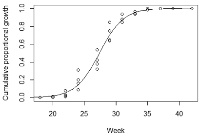
Fig. 1. The cumulative distribution function of the diameter growth of birch within a growing season (line). The function was modeled to estimate the proportion of the growing season that sprouts emerging after early cleaning treatment can still utilize for growth during that year. The initial data (dots) were acquired from Niemistö et al. (2008).
2.6 Statistical analyses
The study’s hypotheses were tested using mixed model analysis. Effects with p-values of less than 0.05 were considered significant. In the EC analysis, the dependent variable was the recorded productive worktime consumed per hectare (pwh ha–1) in the experimental unit (Table 2). The EC1 model was used to test the effects of EC’s season H1) and method (H2), the abundance of ground vegetation cover (H3a), and the elevation changes (H3b) in EC worktime consumption. The covariates in the EC1 model were mean density (1000 trees ha–1), removal diameter (cm), and the logarithmic transformation of the unit’s area. We assumed that the work was slower near the borders of the unit, because the worker had to be careful to stay within the limits of the correct area there. The logarithmic transformation of the area of the experimental unit was considered an appropriate variable to explain the proportion of the area suffering from this hindrance.
In the EC2 model, TWI was added, and direct removal figures were excluded. Otherwise, EC2 was identical to EC1. This was done to identify the effect of TWI on the EC time consumption (H3c). The TWI was considered to indicate the ability of broadleaves to inhabit a site, which is why it was not analyzed in the same model as removal.
In the analysis of PCT time consumption, the dependent variable was the calculated total worktime consumption (twh ha–1). The PCT1 model was used to test the effect of the EC application season on the time consumption of later PCT (H4). The covariates were the same removal figures from 2010 as in the EC1 model. However, the area of the experimental unit was excluded from the covariates, because the time consumption response variable was calculated from removal and did not depend on the experimental unit’s size.
To test the effect of EC on the growth and development of sprouts between EC and forthcoming PCT according to H4, three more models were built: PCTden; PCTdiam; and HRemo. In PCTden and PCTdiam, the density (trees ha–1) or diameter (mm) of removal in PCT was the dependent variable respectively. In PCTden, the logarithmic transformation of the dependent variable was used to correct the heteroscedasticity of residuals’ variance. In Hremo, the dependent variable was the height of the removal divided by the growing seasons after EC. The main effect in these models was the season of EC application. The covariates were the density (trees ha–1) and diameter (mm) of removal during EC. The plot means per experimental unit was used as an observation in the analyses of PCTden and PCTdiam. They were thus analyzed on the same experimental unit level as PCT1. However, Hremo was analyzed at tree level to separate the different tree species in the analysis, including 168 conifers, 375 silver birches, 877 downy birches, 43 aspens, 336 rowans, 125 salixes, and 6 trees of other species.
In the statistical analysis, structural Eq. 2 was used for EC1 and EC2, and structural Eq. 3 was used for PCT1, PCTden, PCTdiam, and Hremo:
![]()
![]()
where Y was the dependent variable; f(·) was the fixed part of the model; x1, x2, …, xn were fixed predictors; and u, v, and e were respectively the random forest worker and site effects, and the error term with a mean of zero and constant variances. The subscript i refers to the experimental unit (or tree in HRemo), and the subscripts j and t refer to the site and forest worker respectively. The variances of the random normally distributed effects and the parameters of fixed predictors were estimated using the statistical software R version 3.5.1 (R Core Team 2018) with the restricted maximum likelihood method (REML) of the lmer function in package lme4 (Bates et al. 2015). All the continuous variables were centered around the mean in all the analyses.
2.7 Cost analysis
The effect of the EC application season and method on the combined costs of EC and PCT was observed in cost analysis. First, the productive work hours (pwh) from EC were converted to total work hours (twh) to correspond to the calculated time consumption in PCT. The average twh/pwh-ratio of 1.65 found in the experimental units was used as a conversion rate.
The total time consumptions were then converted to costs with an hourly multiplier. In the cost analysis, a forest worker’s wage was assumed to be €12.41 twh–1 in accordance with the collective labor agreement in Finland (Metsäalan työehtosopimus... 2018). Direct wage costs were increased by 65.4% to cover the costs of paid days off, pensions and insurance, social security, and other workforce costs (StatFin Online… 2020). Ten percent was then added for supervision costs, and 10% was added as the company’s profit. Finally, €5.61 twh–1 was added for equipment and travel expenses. The total hourly cost of EC and PCT was €30.44 twh–1.
Costs were analyzed as present value analysis with 0–6% discount rates. The present value in the analysis was the time when EC was applied in the spring treatment. In the summer treatment, EC was applied in 0.14 years, and in autumn treatment in 0.39 years, and PCT was applied in all treatments in 4.4 years from the time of calculation.
3 Results
3.1 Time consumption in EC
According to the EC1 model, productive worktime consumption in EC differed between seasons (H1, p < 0.001, Table 3); EC was quickest in the spring (5.3 pwh ha–1), when it took two hours ha–1 less than in the summer (7.3 pwh ha–1) and 0.9 hours ha–1 less than in the autumn (6.2 pwh ha–1). Worktime savings between the spring and summer were 27% in totally cleaned sites and 30% in point cleaned sites. There was also a significant interaction effect between the season and vegetation coverage (H3a, p = 0.024); the differences in time consumption between the seasons were higher the higher the vegetation coverage (Fig. 2). The EC method, whether it was point or total treatment, had no statistically significant effect on the time consumption of EC (H2, p = 0.079). However, point cleaned sites took an average of 0.8 pwh ha–1 less time than totally cleaned sites. Elevation changes had a significant effect on the time consumption of EC (H3b, p = 0.035). The time consumption was higher when the elevation changes were larger, e.g. an increase of 5 m to 20 m increased the time consumption by 0.77 pwh ha–1. The covariates, diameter (p < 0.001), and density (p < 0.001) of the removal, as well as the area of the experimental unit (p < 0.001), were significant variables in the analysis.
| Table 3. Mixed models (EC1 and EC2) for worktime consumption in early cleaning. EC1 is the primary analysis including removal figures as covariates. The secondary analysis (EC2) replaces the direct figures of removal with its indirect indications, the TWI (topographic wetness index) of a site. The worker effect is redundant in EC2, because it cannot be separated from the site-level variation in the model. The dependent variable is worktime consumption in productive working hours (pwh) ha–1 in both models (N = density, D0.15 = diameter at stump height, EC = early cleaning). All the continuous independent variables are centered around the mean. P-values in bold represent statistically significant differences. | ||||||
| EC1 | EC2 | |||||
| Estimate | Std. Error | P-value | Estimate | Std. Error | P-value | |
| Intercept | 5.303 | 0.509 | <0.001 | 5.343 | 0.554 | <0.001 |
| N before EC, 1000 trees ha–1 | 0.175 | 0.015 | <0.001 | |||
| D0.15 before EC, cm | 1.921 | 0.771 | 0.016 | |||
| Season, ref. Spring | ||||||
| Summer | 1.970 | 0.255 | <0.001 | 1.955 | 0.318 | <0.001 |
| Autumn | 0.939 | 0.261 | <0.001 | 0.884 | 0.317 | 0.006 |
| Ln(Area), ha | –1.545 | 0.345 | <0.001 | –1.731 | 0.453 | <0.001 |
| Elevation change, m | 0.256 | 0.119 | 0.035 | 0.103 | 0.167 | 0.538 |
| EC-method, ref. Total cleaning | ||||||
| Point cleaning | –0.774 | 0.412 | 0.079 | –0.742 | 0.689 | 0.293 |
| Vegetation cover, % | –0.017 | 0.027 | 0.516 | –0.005 | 0.033 | 0.892 |
| Season:Vegetation cover, ref. Spring | ||||||
| Summer:Vegetation cover | 0.086 | 0.037 | 0.024 | 0.107 | 0.047 | 0.025 |
| Autumn:Vegetation cover | 0.057 | 0.038 | 0.138 | 0.004 | 0.047 | 0.939 |
| TWI, in thousands | 0.549 | 0.221 | 0.014 | |||
| Random effects | Variance | Std.Dev. | Variance | Std.Dev. | ||
| Stand:Worker | 0.317 | 0.563 | 2.104 | 1.451 | ||
| Worker | 1.267 | 1.126 | 0.000 | 0.000 | ||
| Residual | 1.381 | 1.175 | 2.081 | 1.443 | ||
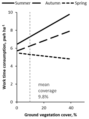
Fig. 2. Estimate of productive worktime consumption in early cleaning in spruce stands according to the EC1 model. Cleanings were applied in different seasons and with varying degrees of ground vegetation coverage. Vegetation cover was determined in the summer or autumn in all treatments, so not necessarily during or close to the application of the treatment. The main effects differed significantly between all seasons. The slope was statistically significant in the summer, but not in the autumn or spring.
The effect of TWI on EC time consumption was tested in the EC2 model (Table 3). The TWI significantly affected the EC time consumption (H3c, p = 0.014). While the range of variation of the TWI was 5720 between experimental sites (Table 2), the time consumption increased by 0.55 pwh ha–1 per 1000 units of the TWI.
3.2 Time consumption in PCT
PCT was applied in the fifth autumn after the EC in all applications—4–5 growing seasons after EC. The season of EC application had a statistically significant effect on the time consumption of PCT (H4, p = 0.016, Table 4). The calculated worktime consumption in PCT was 10.7 twh ha–1, 9.7 twh ha–1, and 10.4 twh ha–1 respectively when EC was applied in the spring, summer, or autumn. PCT was 1 twh ha–1 slower to undertake when EC had been applied in spring instead of summer. Moreover, PCT was only slightly (0.3 twh ha–1) slower to undertake when EC had been applied in spring instead of autumn, even though the time for the removal to grow was basically a growth period longer in the spring treatment.
| Table 4. Mixed models for worktime consumption (model PCT1, total work hours ha–1), removal of density (model PCTden, Ln[trees ha–1]), and diameter of density (model PCTdiam, cm) in PCT in studied spruce stands (N = density, D0.15 = diameter at stump height). All the continuous independent variables are centered around the mean. P-values in bold represent statistically significant differences. | |||||||||
| PCT1 | PCTden a | PCTdiam | |||||||
| Estimate | Std. Error | P-value | Estimate | Std. Error | P-value | Estimate | Std. Error | P-value | |
| Intercept | 10.698 | 0.521 | <0.001 | 2.940 | 0.102 | <0.001 | 1.368 | 0.062 | <0.001 |
| Season, ref. Spring | |||||||||
| Summer | –1.000 | 0.410 | 0.016 | –0.136 | 0.066 | 0.043 | –0.091 | 0.062 | 0.146 |
| Autumn | –0.291 | 0.421 | 0.490 | –0.014 | 0.069 | 0.839 | –0.112 | 0.064 | 0.082 |
| EC-method, ref. Total cleaning | |||||||||
| Point cleaning b | –1.456 | 0.622 | 0.028 | –0.241 | 0.126 | 0.068 | 0.099 | 0.068 | 0.158 |
| N before EC, 1000 trees ha–1 | 0.200 | 0.023 | <0.001 | 0.041 | 0.004 | <0.001 | –0.012 | 0.003 | <0.001 |
| D0.15 before EC, cm | –1.503 | 1.191 | 0.212 | –0.125 | 0.218 | 0.566 | –0.103 | 0.144 | 0.482 |
| Random effects: | Variance | Std.Dev. | Variance | Std.Dev. | Variance | Std.Dev. | |||
| Stand | 1.244 | 1.116 | 0.007 | 0.086 | 0.007 | 0.086 | |||
| Residual | 3.725 | 1.930 | 0.086 | 0.293 | 0.086 | 0.293 | |||
| a) Log-transformed dependent variable used in PCTden. b) It should be noted that placement of experiment plots differed between EC methods (see discussion). | |||||||||
On average, PCT took 10.7 twh ha–1 and 9.2 twh ha–1 respectively in totally and point cleaned sites. The calculated time consumption in PCT was 1.5 twh ha–1 lower in point cleaned sites (p = 0.028).
3.3 Development of removal between EC and PCT
A closer analysis of removal in PCT indicated that the season of EC application had a statistically significant effect on density (p = 0.043), but not on the diameter (p = 0.146) of removal (Table 4). The density of removal was 13.6% lower in PCT if EC had been applied in the summer instead of the spring. This corresponds to 2557 trees ha–1, with an average density of 18 800 trees ha–1 in the study. The difference in density was negligible between the spring and autumn treatments. The EC method did not have a significant effect either on the density (p = 0.068) or removal diameter (p = 0.158), even though the average density of removal was 24.1% lower in point cleaned sites than in totally cleaned sites. The average removal diameter in PCT was only 0.1 cm higher in point cleaned sites than in totally cleaned sites (when the sample was taken from the five closest trees of a crop tree in a point cleaned site).
The height of the removal in PCT divided by the growing seasons between EC and PCT, hereafter referred to as the height growth of removal, was significantly influenced by the season when EC was applied (p < 0.001, Table 5). Removal grew most slowly when EC was applied in the spring, at 34.2 cm year–1 (Fig. 3). The growth of removal was about the same when EC was applied in the summer, at 34.6 cm year–1. In contrast, removal grew much more quickly when cleaning was applied in autumn, at 41.9 cm year –1. The EC method did not have a significant effect on the growth of removal, even though it was a little higher in point cleaned sites on average (Table 5, Fig. 3). Different tree species in removal grew at significantly different speeds. Excluding the “Other” category, silver birch was the fastest growing species in removal, but it grew only 0.4 cm year–1 more quickly than pubescent birch (Fig. 4). The difference between birches was non-significant. Aspen grew most slowly, followed by rowan. The initial density of the stand before EC was a significant covariate in the analysis, but the diameter was not.
| Table 5. Mixed model (Hremo) for height growth (cm year–1) of the removal between early cleaning (EC) and pre-commercial thinning (PCT) in spruce stands studied in southern Finland (N = density, D0.15 = diameter at stump height). All the continuous independent variables are centered around the mean. P-values in bold represent statistically significant differences. | |||
| Estimate | Std. Error | P-value | |
| Intercept | 34.190 | 1.814 | <0.001 |
| Season, ref. Spring | |||
| Summer | 0.397 | 0.345 | 0.249 |
| Autumn | 7.669 | 0.361 | <0.001 |
| EC-method, ref. Total cleaning | |||
| Point cleaning | 2.554 | 2.338 | 0.286 |
| Species, ref. Downy birch | |||
| Conifer | –1.417 | 0.544 | 0.009 |
| Silver birch | 0.432 | 0.461 | 0.349 |
| Aspen | –5.966 | 1.015 | <0.001 |
| Other | 7.850 | 2.571 | 0.002 |
| Sorbus | –2.025 | 0.438 | <0.001 |
| Salix | –1.795 | 0.615 | 0.004 |
| N before EC, 1000 trees ha–1 | –0.142 | 0.033 | <0.001 |
| D0.15 before EC, cm | 2.367 | 1.514 | 0.118 |
| Random effects: | Variance | Std.Dev. | |
| Stand | 28.350 | 5.324 | |
| Residual | 38.110 | 6.173 | |
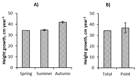
Fig. 3. Post early cleaning (EC) growth rate of the trees removed in pre-commercial thinning (mainly resprouts from EC) according to the season of application (A) or the method (B) of EC in the studied spruce stands. The error bars are the 95% confidence intervals of the parameter estimates compared to the reference category (Spring in A or Total in B) in the Hremo model.
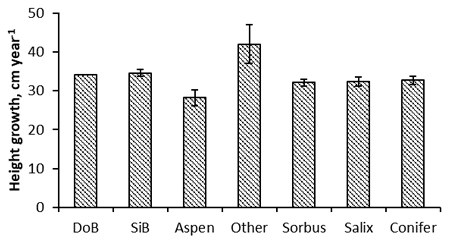
Fig. 4. Post early cleaning growth rate of the trees of different species removed in pre-commercial thinning (mainly resprouts from EC) of the studied spruce stands (DoB = downy birch, SiB = silver birch). The error bars are the 95% confidence intervals of the parameter estimates compared to the reference category (DoB) in the Hremo model.
3.4 Time consumption and costs in a juvenile stand management program
At the management program level, we analyzed the time consumption and costs of juvenile stand management for totally cleaned sites, which was considered more valid than for point cleaned sites. The juvenile stand management program was most efficient when EC was applied in the spring; the combined time consumption of EC and PCT was then 19.4 twh ha–1 (Fig. 5). It increased by 2.3 twh ha–1 or 1.3 twh ha–1 respectively when EC was applied in the summer or autumn.
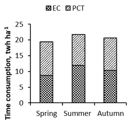
Fig. 5. The effect of the season of application of early cleaning (EC) on the time consumption of the juvenile stand management program in total working hours (twh) ha–1, i.e. on the combined time consumption of EC and 4–5 growing seasons later following pre-commercial thinning (PCT).
With a 3% interest rate, the discounted costs of EC as total cleaning in the summer and PCT were €623 ha–1 (Table 6). Applying EC in the spring instead accounted for savings of 11% at the juvenile stand management program level: The costs were €522 ha–1. Applying different discount rates (0–6%) had only a minor effect on the differences between management programs.
| Table 6. Costs of early cleaning (EC) and pre-commercial thinning (PCT) with a nominal rate (0%) and with a 3% discounted rate in totally cleaned and point cleaned spruce stands when cleaning was applied in the spring, summer, or autumn. The present values have been calculated to the timepoint when the first EC treatment was applied in the spring. | |||||
| EC, € ha–1 | PCT, € ha–1 | Overall, € ha–1 | EC time, years | PCT time, years | |
| Nominal rate, 0% | |||||
| Spring - Total | 266 | 326 | 592 | ||
| Summer - Total | 365 | 295 | 661 | ||
| Autumn - Total | 313 | 317 | 630 | ||
| Discount rate, 3% | |||||
| Spring - Total | 266 | 312 | 578 | 0.00 | 4.40 |
| Summer - Total | 365 | 283 | 647 | 0.14 | 4.40 |
| Autumn - Total | 312 | 303 | 615 | 0.39 | 4.40 |
4 Discussion
In this study, we observed the different applications of a multistage juvenile stand management program on the time consumption of EC and PCT operations. The focus was especially on the first stage of the program, EC, the methods, and the season in which it was applied.
As we hypothesized (H1), the EC application season influenced the associated time consumption. Depending on the cleaning method, the seasonal timing of EC could contribute to worktime consumption fluctuations of between 27 and 30%. Uotila et al. (2020) found a similar difference in worktime fluctuations between seasons in cross-sectional data. In small cross-sectional data, Hämäläinen and Kaila (1983) also found that PCT in the spring was more productive than in the summer. The most productive time for EC seems to be the spring, followed by the autumn. Summer is the least productive; there is great coherence in these three studies on this point.
We hypothesized that time consumption in EC differed between the applied cleaning methods—total cleaning or point cleaning (H2). In point cleaned sites, the time consumption was 0.8 pwh ha–1 lower than in totally cleaned sites, but the difference was insignificant (p = 0.079). The difference is rational, but larger or more specific data on this topic are needed to confirm the result. This study was primarily designed to identify the differences between EC application seasons, not as precisely the differences between EC methods. The few studies that address this topic have found no consistent differences between the time consumption of point cleaning and total cleaning. Saksa and Miina (2010) found that point cleaning took 40% less time than total cleaning in 1–2-meter-high Scots pine stands, but there were no differences in 3-meter-high stands. Furthermore, Miina and Saksa (2013) found no significant differences in the time consumption of EC between cleaning methods in Scots pine stands. These two studies by Miina and Saksa estimated time consumption with models based on removal, why the results only reflect the differences in the number and size of the removed trees.
In this study, we also found that ground vegetation played a role in how much the season affected the time consumption of EC (H3a). In the summer, the time consumption of EC increased heavily with an increasing amount of ground vegetation. The effect was significant. In the spring, the time consumption decreased with an increasing amount of ground vegetation, though the decline was not significant. Vegetation cover was determined in the summer or autumn for all treatments, not necessarily during or close to the application of EC. Sites that were observed to have a large amount of ground vegetation may therefore be quicker to clean in the spring with the fallen herbs on them than sites with a small amount of ground vegetation, which lack the effect of fallen herbs leveling the ground. Nevertheless, in the spring, ground vegetation seems to have little influence on time consumption in EC, whereas in the summer, it greatly increases the time consumption in EC.
We also found that the time consumption of EC depended on the elevation changes (H3b) and wetness of a site (H3c). Similar findings have previously been observed with elevation changes in Hämäläinen and Kaila (1983), and with wetness in Uotila et al. (2020).
The PCT time consumption was estimated in the fifth autumn after the EC in all treatments. The time interval between EC and PCT was therefore a little longer the earlier EC was applied. Yet the time consumption in PCT was lowest when EC was applied in the summer. This was in accordance with H3, that time consumption in PCT differed between EC application seasons. The reason for this has been well described by the literature. Stumps established during the growing season typically sprout less intensively than stumps cut in the dormant season (Stoeckeler 1947; Belanger 1979; Strong and Zavitkovski 1983; Harrington 1984; DeBell and Turpin 1989; Dickmann and Pregitzer 1992; Bell et al. 1999; Xue et al. 2013).
In our analysis of annual height growth, we discovered that sprouts cut in the summer grew more slowly than those cut in the autumn (H5). However, sprouts cut in the spring grew even more slowly than those cut in the summer, though the difference was non-significant (p = 0.249). The low growth of spring-cut sprouts may often have been unnoticed because of the varying time interval between applications and the focus on the height of the sprouts; sprouts cut in the spring are typically longer than those cut in the summer (Etholén 1974; Ferm and Issakainen 1981; Johansson 1992c), but they may still have grown more slowly. For example, Etholén (1974) found that the sprouts of birch or aspen cut in the early summer were taller than those cut in the autumn when they were measured the following autumn. However, the third autumn after the cutting, the sprouts cut in the autumn seemed to reach the height of those cut in the early summer. Furthermore, Heikinheimo (1930) found that four growing seasons after the cutting year, gray alders cut in the spring to early summer were shorter than those cut later in the summer or autumn. However, the sprouting of broadleaves may greatly depend on weather conditions, so the effect of the cutting time can vary somewhat between years (Etholén 1974; Ferm and Issakainen 1981). Moreover, in this study, individual tree growth should have been measured to draw stronger conclusions on the differences in the growth of the trees in the treatments.
After EC, silver birch was the fastest growing species among removal trees, whereas aspens grew slowest, followed by rowan. According to Härkönen (1998), aspen and rowan are very susceptible to moose browsing, which explains why this result may indicate the vulnerability of aspen and rowan to browsing rather than their tendency to grow slowly after EC. However, at least in heavily browsed areas, birch can constitute one of the highest risks for the renewal of juvenile stand management through sprouting.
In this study, point cleaned sites were less time consuming in PCT than totally cleaned sites. However, sampling in the latter measurement (2014–2015) differed between point cleaned and totally cleaned sites. In totally cleaned sites, the plots were systematically set at the sampling line, but in point cleaned sites the center of the plots was assigned typically slightly apart from the line to the nearest crop tree. This approach was likely to cause some sampling bias between cleaning methods, especially in the removal diameter. The cleaning method was therefore excluded from the management program level analyses. In our data, the diameter in PCT was one millimeter larger, and time consumption 16% higher, in point cleaned sites than in totally cleaned sites. In Saksa and Miina (2013), the removal diameter in PCT was 4–17 mm larger, and the time consumption of PCT was 11–82% higher, in point cleaned Scots pine sites than in totally cleaned sites.
The density of removal had the highest impact on EC time consumption among the analyzed variables. The removal diameter also significantly affected EC time consumption. Density and size, either diameter or height, are basically included in all the models previously constructed to estimate the time consumption of PCT in the field (Hämäläinen and Kaila 1983; Bergstrand et al. 1986; Kaila et al. 2006; Ligne et al. 2005; Lebel et al. 2007). These results were therefore expected. Although it should be noticed that the removal figures were susceptible to sampling error. The removal sample was measured from 0.4–3.8% of the total treatment area in EC. In PCT, the sample was 2.5 times larger than in EC, covering 1.0–8.4% of the treatment unit, which improved the precision of the models when removal variables were used as dependent variables, i.e. in PCT. Although the sample represented a small area of the experiment units, the total dataset of 132 units was quite large, and the standard error for removal density remained low in estimating EC time consumption, e.g. in the EC1 model. Moreover, the stands had been carefully selected to represent the stage of EC, and the general classification of the sites in forest management planning emphasizes the sites’ homogeneity.
As a practical implication, the results suggest that the spring or autumn is a good time to implement EC. A general application in practice is to undertake EC in the summer with total cleaning, which proved the most expensive of the observed alternatives in this study. Cost savings through less intense sprouting are often cited as one of the reasons for conducting EC in summer. However, the time savings from EC in the spring (27%) or autumn (14%) were so big that they compensated or more than compensated the better growth of sprouts and the additional costs it caused in PCT. EC in the spring saved 11% of total juvenile stand management costs (including EC and PCT). EC in the autumn was also a little less expensive on a management program level than EC in the summer. There is therefore no reason to avoid EC in the autumn either. These results are applicable only when the land is not covered by snow.
In the present study, the worktime savings from different seasons were observed in EC. However, it is also likely that the savings are similar or a little smaller between application seasons in later PCT, as described by Uotila et al. (2020). Within workforce limitations, it is therefore rational for those sites which have poor visibility because of vegetation in the summer to be early cleaned or pre-commercially thinned in the spring or even autumn. Furthermore, workforce resource allocation should be reconsidered, given that juvenile stand management is efficient in the spring. We can expect gains in forestry with these procedures throughout boreal spruce forests.
In conclusion, according to H1, EC time consumption differed between seasons, and EC was the least time consuming in the spring, followed by the autumn. It was most time consuming in the summer. The time consumption in EC also differed between cleaning methods (H2). Point cleaning consumed less time than total cleaning. Site conditions such as ground vegetation (H3a), elevation changes (H3b), and site wetness (H3c) influenced EC time consumption. The time consumption in consequent PCT depended on the initial EC application season (H4), and it was least time consuming when EC was applied in the summer. The season of EC influenced the development of removal between EC and PCT (H5). The growth of the sprout was slowest when EC was applied in the spring, and the density was lowest when EC was applied in the summer. The juvenile stand management program was least expensive when EC was applied in the spring, followed by the fall. It was most expensive when EC was applied in the summer.
Acknowledgments
We are grateful to the two reviewers of this article’s manuscript. Their thoughtful comments and constructive feedback enabled us to improve the article in many areas.
Declaration of openness of research materials, data, and code
The data and code used in the analyses are available on request from karri.uotila@luke.fi. The materials used and their availability are described in the article text.
References
Andersson B (1993) Lövträdens inverkan på små tallars (Pinus sylvestris) överlevnad, höjd och diameter. [Effect of broadleaves on survival, height and diameter of a small pine]. Rapporter 36, Sveriges Landbruksuniversitet, Institutionen för Skogsskötsel.
Bates D, Mächler M, Bolker BM, Walker SC (2015) Fitting linear mixed-effects models using lme4. J Stat Softw 67: 1–48. https://doi.org/10.18637/jss.v067.i01.
Belanger RP (1979) Stump management increases coppice yield of sycamore. South J Appl For 3: 101–103. https://doi.org/10.1093/sjaf/3.3.101.
Bell FW, Pitt DG, Morneault AE, Pickering SM (1999). Response of immature trembling aspen to season and height of cut. North J Appl For 16: 108–114. https://doi.org/10.1093/njaf/16.2.108.
Beven KJ, Kirkby MJ (1979) A physically based variable contributing area model of basin hydrology. Hydrolog Sci J 24: 43–69. https://doi.org/10.1080/02626667909491834.
Cajander AK (1926) The theory of forest types. Acta For Fenn 29. https://doi.org/10.14214/aff.7193.
DeBell DS, Turpin TC (1989) Control of red alder by cutting. Research Paper PNW-RP-414, USDA, Forest Service, Pacific Northwest Research Station, Portland, OR, USA. https://doi.org/10.2737/PNW-RP-414.
Dickmann DI, Pregitzer KS (1992) The structure and dynamics of woody plant root systems. In: Mitchell CP, Ford-Robertson JB, Hinkley T, Sennery-Forsse L (eds) Ecophysiology of short rotation forest crops. Springer Netherlands, pp 95–123. ISBN 978-1-85166-848-9.
Etholén K (1974) Kaatoajankohdan vaikutus koivun ja haavan vesomiseen taimistonhoitoaloilla Pohjois-Suomessa. Summary: The effect of felling time on the sprouting of Betula pubescens and Populus tremula in the seedling stands in Northern Finland. Folia For 213. http://urn.fi/URN:ISBN:951-40-0127-3.
Fairdata.fi (2020) Topographical wetness index for Finland, 16m, 2016. https://etsin.fairdata.fi/dataset/e1206dd8-e74d-46ff-b202-54db3f1a8778. Accessed 3 Aug 2020.
Ferm A, Issakainen J (1981) Kaatoajankohdan ja kaatotavan vaikutus hieskoivun vesomiseen turvemaalla. Metsäntutkimuslaitoksen tiedonantoja 33. http://urn.fi/URN:NBN:fi-metla-201207201924.
Ferm A, Kauppi A, Rinne P, Tela H-L, Saarsalmi A, Sevola Y (1985) Energiapuun tuottaminen luonnonvesakoissa. Summarry: The potential of forest energy in Finland. In: Hakkila P (ed) Metsäenergian mahdollisuudet Suomessa. PERA-projektin väliraportti. Folia For 624: 29–44. http://urn.fi/URN:ISBN:951-40-0704-2.
Folkesson B, Bärring U (1982) Exempel på en riklig björkförekomst inverkan på utvecklingen av unga tall- och granbestånd i norra Sverige. Abstract: Some examples of the influence of an abundant occurrence of birch on the development of young Norway spruce and Scots pine stands in north Sweden. Rapport 1, Sveriges lantbruksuniversitet, avdelning för skoglig herbologi.
Hämäläinen J, Kaila S (1983) Taimikon perkauksen ja harvennuksen sekä uudistusalan raivauksen ajanmenekkisuhteet. [Time expenditure on cleaning and thinning of young stands and clearing of cutting areas by brush saw]. Metsätehon katsaus 16/1983. https://metsateho.fi/wp-content/uploads/katsaus-1983_16.pdf. Accessed 3 Aug 2020.
Härkönen S (1998) Effects of silvicultural cleaning in mixed pine‐deciduous stands on moose damage to scots pine (Pinus sylvestris). Scand J Forest Res 13: 429–436. https://doi.org/10.1080/02827589809383003.
Harrington CA (1984) Factors influencing initial sprouting of red alder. Can J Forest Res 14: 357–361. https://doi.org/10.1139/x84-065.
Heikinheimo O (1930) Kaatoajan vaikutus lehtipuiden vesojen syntyyn ja kasvuun. [Effect of felling time on sprouting of broadleaved trees]. Keskusmetsäseura Tapio, Helsinki, pp 113–117.
Huuskonen S, Haikarainen S, Sauvula-Seppälä T, Salminen H, Lehtonen M, Siipilehto J, Ahtikoski A, Korhonen KT, Hynynen J (2020) Benefits of juvenile stand management in Finland – impacts on wood production based on scenario analysis. Forestry 93: 458–470. https://doi.org/10.1093/forestry/cpz075.
Hytönen J (2019) Stump diameter and age affect coppicing of downy birch (Betula pubescens Ehrh.). Eur J For Res 138: 345–352. https://doi.org/10.1007/s10342-019-01175-5.
Hytönen J, Issakainen J (2001) Effect of repeated harvesting on biomass production and sprouting of Betula pubescens. Biomass Bioenergy 20: 237–245. https://doi.org/10.1016/S0961-9534(00)00083-0.
Johansson T (1987) Development of stump suckers by Betula pubescens at different light intensities. Scand J Forest Res 2: 77–83. https://doi.org/10.1080/02827588709382447.
Johansson T (1992a) Dormant buds on Betula pubescens and Betula pendula stumps under different field conditions. Forest Ecol Manag 47: 245–259. https://doi.org/10.1016/0378-1127(92)90277-G.
Johansson T (1992b) Sprouting of 10- to 50-year-old Betula pubescens in relation to felling time. Forest Ecol Manag 53: 283–296. https://doi.org/10.1016/0378-1127(92)90047-D.
Johansson T (1992c) Sprouting of 2- to 5-year-old birches (Betula pubescens Ehrh. And Betula pendula Roth) in relation to stump height and felling time. Forest Ecol Manag 53: 263–281. https://doi.org/10.1016/0378-1127(92)90046-C.
Johansson T (2008) Sprouting ability and biomass production of downy and silver birch stumps of different diameters. Biomass Bioenergy 32: 944–951. https://doi.org/10.1016/j.biombioe.2008.01.009.
Kaila S, Kiljunen N, Miettinen A, Valkonen S (2006) Effect of precommercial thinning on the consumption of working time in Picea abies stands in Finland. Scand J Forest Res 21: 496–504. https://doi.org/10.1080/02827580601073263.
LeBel LG, Dubeau D (2007) Predicting the productivity of motor-manual workers in precommercial thinning operations. Forest Chron 83: 215–220. https://doi.org/10.5558/tfc83215-2.
Ligné D, Eliasson L, Nordfjell T (2005) Time consumption and damage to the remaining stock in mechanised and motor manual pre-commercial thinning. Silva Fenn 39: 455–464. https://doi.org/10.14214/sf.379.
Luoranen J, Saksa T, Uotila K (2012) Metsän uudistaminen. [Forest regeneration]. Metsäkustannus Oy, Hämeenlinna.
Metsäalan työehtosopimus 1.2.2018–31.1.2020 (2008) [Collective labor agreement on forestry 2018]. Maaseudun Työnantajaliitto, Metsähallitus, Metsäteollisuus ry, Yksityismetsätalouden Työnantajat, Teollisuusliitto.
Miina J, Saksa T (2013) Perkauksen vaikutus männyn kylvö- ja luontaisen taimikon kehitykseen ja taimikonhoidon ajanmenekkiin. [The effect of early cleaning on stand development and time consumption in pre-commercial thinning in direct-seeded and naturally established scots pine stands]. Metsätieteen aikakauskirja 1/2013: 33–44. https://doi.org/10.14214/ma.6030.
Mikola P (1942) Koivun vesomisesta ja sen metsänhoidollisesta merkityksestä. [Sprouting of birch and the silvicultural importance of it]. Acta For Fenn 50. https://doi.org/10.14214/aff.7356.
Onorfi A (2019) Some useful equations for nonlinear regression in R. https://www.statforbiology.com/nonlinearregression/usefulequations. Accessed 3 Aug 2020.
Salmivaara A, Launiainen S, Tuominen S, Ala-Ilomäki J, Finér L (2017) Topographic wetness index for Finland. Natural Resources Institute Finland, Etsin research data finder. https://etsin.avointiede.fi/.
Saksa T, Miina J (2007) Cleaning methods in planted Scots pine stands in southern Finland: 4-year results on survival, growth and whipping damage of pines. Silva Fenn 41: 661–670. https://doi.org/10.14214/sf.274.
Saksa T, Miina J (2010) Perkaustavan ja -ajankohdan vaikutus männyn istutustaimikon kehitykseen Etelä-Suomessa. [The effect of the method and timing of cleaning on the development of planted Scots pine stand]. Metsätieteen aikakauskirja 2/2010: 115–127. https://doi.org/10.14214/ma.5738.
StatFin Online Service (2020) Structure of labour costs by labour market sector. https://pxnet2.stat.fi/PXWeb/pxweb/en/StatFin/StatFin__pal__tvtutk/statfin_tvtutk_pxt_001.px. Accessed 3 Aug 2020.
Stoeckeler JH (1947) When is plantation release most effective? Journal of Forestry 45: 265–271. https://doi.org/10.1093/jof/45.4.265.
Strong T, Zavitkovski J (1983) Effect of harvesting season on hybrid poplar coppicing. In: Hansen EA (ed) Intensive plantation culture: 12 years research. General Technical Report NC-91, USDA, Forest Service Northern Central Forest Experimental Station, Saint Paul, MN, USA, pp 54–57. https://doi.org/10.2737/NC-GTR-91.
Uotila K (2017).Optimization of early cleaning and precommercial thinning methods in juvenile stand management of Norway spruce stands. Diss For 231. https://doi.org/10.14214/df.231.
Uotila K, Rantala J, Saksa T, Harstela P (2010). Effect of soil preparation method on economic result of Norway spruce regeneration chain. Silva Fenn 44: 511–524. https://doi.org/10.14214/sf.146.
Uotila K, Miina J, Saksa T, Store R, Kärkkäinen K, Härkönen M (2020) Low cost prediction of time consumption for pre-commercial thinning in Finland. Silva Fenn 54, article id 10196. https://doi.org/10.14214/sf.10196.
Xue Y, Zhang W, Zhou J, Ma C, Ma L (2013) Effects of stump diameter, stump height, and cutting season on Quercus variabilis stump sprouting. Scand J Forest Res 28: 223–231. https://doi.org/10.1080/02827581.2012.723742.
Walfridsson E (1976) Lövets konkurrens i barrkulturen. [Competition of broad-leaved trees in coniferous plantations]. Skogen 63: 631–633.
Total of 44 references.
