Miro Demol  ,
Phil Wilkes,
Pasi Raumonen,
Sruthi M. Krishna Moorthy,
Kim Calders,
Bert Gielen,
Hans Verbeeck
,
Phil Wilkes,
Pasi Raumonen,
Sruthi M. Krishna Moorthy,
Kim Calders,
Bert Gielen,
Hans Verbeeck
Volumetric overestimation of small branches in 3D reconstructions of Fraxinus excelsior
Demol M., Wilkes P., Raumonen P., Krishna Moorthy S. M., Calders K., Gielen B., Verbeeck H. (2022). Volumetric overestimation of small branches in 3D reconstructions of Fraxinus excelsior. Silva Fennica vol. 56 no. 1 article id 10550. https://doi.org/10.14214/sf.10550
Highlights
- We compare branch diameter and tree woody volume estimates from terrestrial laser scanning data with manual measurements of two Fraxinus excelsior trees
- Smaller branch diameters are generally overestimated due to scattering and misalignment errors in the point cloud
- Consequently, tree woody volume is overestimated by 38% to 52%
- Filtering by reflectance and improved alignment partly mitigate this effect.
Abstract
Terrestrial laser scanning (TLS) has been applied to estimate forest wood volume based on detailed 3D tree reconstructions from point cloud data. However, sources of uncertainties in the point cloud data (alignment and scattering errors, occlusion, foliage...) and the reconstruction algorithm type and parameterisation are known to affect the reconstruction, especially around finer branches. To better understand the impacts of these uncertainties on the accuracy of TLS-derived woody volume, high-quality TLS scans were collected in leaf-off conditions prior to destructive harvesting of two forest-grown common ash trees (Fraxinus excelsior L.; diameter at breast height ~28 cm, woody volume of 732 and 868 L). We manually measured branch diameters at 265 locations in these trees. Estimates of branch diameters and tree volume from Quantitative Structure Models (QSM) were compared with these manual measurements. The accuracy of QSM branch diameter estimates decreased with smaller branch diameters. Tree woody volume was overestimated (+336 L and +392 L) in both trees. Branches measuring < 5 cm in diameter accounted for 80% and 83% of this overestimation respectively. Filtering for scattering errors or improved coregistration approximately halved the overestimation. Range filtering and modified scanning layouts had mixed effects. The small branch overestimations originated primarily in limitations in scanner characteristics and coregistration errors rather than suboptimal QSM parameterisation. For TLS-derived estimates of tree volume, a higher quality point cloud allows smaller branches to be accurately reconstructed. Additional experiments need to elucidate if these results can be generalised beyond the setup of this study.
Keywords
aboveground biomass;
crown architecture;
LIDAR;
quantitative structure models;
common ash;
woody tree volume
-
Demol,
CAVElab – Computational and Applied Vegetation Ecology, Department of Environment, Faculty of Bioscience Engineering, Ghent University, Coupure Links 653, B-9000 Ghent, Belgium; PLECO – Plants and Ecosystems, Faculty of Science, Antwerp University, Universiteitsplein 1, B-2610 Wilrijk, Belgium
 https://orcid.org/0000-0002-5492-2874
E-mail
miro.demol@ugent.be
https://orcid.org/0000-0002-5492-2874
E-mail
miro.demol@ugent.be
-
Wilkes,
UCL Department of Geography, Gower Street, London WC1E 6BT, UK; NERC National Centre for Earth Observation (NCEO), UK
https://orcid.org/0000-0001-6048-536X
E-mail
p.wilkes@ucl.ac.uk
-
Raumonen,
Mathematics, Tampere University, FI-33101 Tampere, Finland
https://orcid.org/0000-0001-5471-0970
E-mail
pasi.raumonen@tuni.fi
-
Krishna Moorthy,
CAVElab – Computational and Applied Vegetation Ecology, Department of Environment, Faculty of Bioscience Engineering, Ghent University, Coupure Links 653, B-9000 Ghent, Belgium
https://orcid.org/0000-0002-6838-2880
E-mail
Sruthi.KrishnaMoorthyParvathi@ugent.be
-
Calders,
CAVElab – Computational and Applied Vegetation Ecology, Department of Environment, Faculty of Bioscience Engineering, Ghent University, Coupure Links 653, B-9000 Ghent, Belgium
https://orcid.org/0000-0002-4562-2538
E-mail
kim.calders@ugent.be
-
Gielen,
PLECO – Plants and Ecosystems, Faculty of Science, Antwerp University, Universiteitsplein 1, B-2610 Wilrijk, Belgium
https://orcid.org/0000-0002-4890-3060
E-mail
bert.gielen@uantwerpen.be
-
Verbeeck,
CAVElab – Computational and Applied Vegetation Ecology, Department of Environment, Faculty of Bioscience Engineering, Ghent University, Coupure Links 653, B-9000 Ghent, Belgium
https://orcid.org/0000-0003-1490-0168
E-mail
hans.verbeeck@ugent.be
Received 5 April 2021 Accepted 17 January 2022 Published 28 January 2022
Views 71195
Available at https://doi.org/10.14214/sf.10550 | Download PDF

Supplementary Files
1 Introduction
In the past decade, terrestrial laser scanning (TLS) has matured from an experimental tool into an established instrument in forest mensuration (Calders et al. 2020). One of the most disruptive applications in quantitative forestry is the geometrical reconstruction of point clouds into realistic 3D models of trees, commonly referred to as Quantitative Structure Models (QSMs). This allowed, for the first time, to directly assess several key forest features in a non-destructive and 3D explicit way. The QSM reconstruction algorithms such as TreeQSM (Raumonen et al. 2013), SimpleTree (Hackenberg et al. 2015a), AdTree (Du et al. 2019), and 3DForest (Trochta et al. 2017) have been used to acquire the aboveground woody volume (including all live and dead standing wood, but excluding foliage, fruits, flowers) of standing trees with minimal user input. Wood density allowed to convert QSM volume into aboveground woody biomass (AGB) (Momo et al. 2020). Several experiments have tested the accuracy of TLS-derived estimates of tree volume and AGB against destructive data of full tree measurements (Table 1).
| Table 1. Aboveground woody biomass (AGB) validation experiments comparing terrestrial laser scanned biomass estimates with destructively assessed biomass. Beam exit diameter and beam divergence from RIEGL Laser Measurement Systems GmbH (2020), Momo Takoudjou et al. (2017) and Faro Technologies Inc. (2009). The foliage column indicates if, at the time of scanning, needles or leaves were present. n: number of trees. Some authors have removed leaves from leaf-on point clouds prior to QSM generation. ‘Tree parts’ details which parts of the tree were compared between scans and destructive measurements. Full tree: all above ground parts, leafs excluded. In two cases, an upper branch diameter limit was used such that QSMs were pruned to the threshold diameter. The reported aggregated bias in aboveground biomass (AGB) estimate with TLS with respect to destructive values is shown in percentage. Volume estimates were obtained with SimpleTree a, TreeQSM b and voxelisation c (sensu Bienert et al. 2014). One case d compared full tree destructive AGB with >5 cm diameter TLS-derived AGB. | |||||||
| Reference | Scanner | Beam exit diameter and divergence (mm, mrad) | Foliage | n | Leaf stripping | Tree parts | Plot AGB bias |
| Calders et al. (2015) | RIEGL VZ-400 | 7, 0.35 | Leaf-on | 65 | No | Full tree | +9.68% b |
| Hackenberg et al. (2015a) | Z+F IMAGER 5010 | - | Leaf-off | 12 | No | Full tree | +2.42% a +19.6% b |
| Hackenberg et al. (2015a) | Z+F IMAGER 5010 | - | Leaf-on | 12 | Intensity thresholding + Eucl. Clustering | Full tree | +3.6% a –0.6% b |
| Hackenberg et al. (2015a) | Z+F IMAGER 5010 | - | Needle-on | 12 | Intensity thresholding + NN | Full tree | –17.0% a –4.6% b |
| Momo Takoudjou et al. (2017) | Leica C10 Scanstation | 4.5, 0 | Leaf-on | 61 | Manual | > 5 cm diameter | +5.2%a |
| Burt et al. (2021) | RIEGL VZ-400 | 7, 0.35 | Leaf-on | 4 | TLSeparation v1.2.1.5 | Full tree | –0.8% b |
| Gonzalez de Tanago et al. (2018) | RIEGL VZ-400 | 7, 0.35 | Leaf-on | 29 | No | > 10 cm diameter | –3.7%b |
| Kunz et al. (2017) | FARO Photon 120 | 3.3, 0.16 | Leaf-off | 24 | No | Full tree | –0.8% c –5.5% b –17.3% a |
| Thesis (Burt 2017) | RIEGL VZ-400 | 7, 0.35 | Leaf-off Leaf-on | 3 | No No | > 5 cm diameter | +3.7% b,d +26% b,d |
| Lau et al. (2019) | RIEGL VZ-400 | 7, 0.35 | Leaf-on | 26 | TLSeparation | Full tree | +2.9%b |
| Kükenbrink et al. (2021) | RIEGL VZ-1000 | 7, 0.35 | Almost leaf-off | 55 | Manual, few trees | Full tree | –9.5% |
For plot-aggregated estimates of AGB, prediction errors of QSM-derived AGB range from –4.6% to 26% across many scanning conditions, scanner types and reconstruction algorithms (Table 1). It is notably more challenging to assess the performance of QSMs to reconstruct individual trees or tree parts. An outstanding issue lies in obtaining reliable reconstructions of small branches, which often go unnoticed on the scale of the full tree assessment or plot-level averages. Lau et al. (2018) found that for branches of nine tropical trees measuring 10–20 cm in stem diameter that less than half of the branches could be reconstructed. For the reconstructed branches, branch diameter was overestimated by 40% on average. Smaller branches also had a larger relative overestimation. Additionally, Hackenberg et al. (2015b) demonstrated an increasing tree volume overestimation as smaller branches (10, 7, 4 cm diameter) in QSM reconstructions were included. To cope with overestimations, some authors remove the smallest branches in the reconstructions based on a minimum diameter threshold: Burt (2017) (5 cm threshold); Momo Takoudjou et al. (2017) (5 cm); Gonzalez de Tanago et al. (2018) (10 cm); Dassot et al. (2012) (7 cm). The presence of foliage is another element that introduces uncertainty in branch reconstructions (Vicari et al. 2019).
Pyörälä et al. (2018, 2019) and Lau et al. (2019) quantitatively validated TLS-derived branch diameters for boreal and tropical trees respectively. Wilkes et al. (2021) performed an indoor experiment to assess the accuracy of small-branch reconstructions. However, no experiments have destructively validated individual branch diameter reconstruction accuracy of branches smaller than < 10 cm in field conditions. At the same time, the accuracy of branch dimensions in QSM reconstructions is a prerequisite in many applications beyond solely quantifying tree volume or forest AGB. QSM is being used for studying volume allocation patterns (Ver Planck and MacFarlane 2014), crown architecture (Lau et al. 2018), fundamental tree ecology (Lehnebach et al. 2018), volume of lianas (Krishna Moorthy et al. 2020b), structural branch properties (Jackson et al. 2019), surface area of branches (Van Langenhove et al. 2021), volume expansion factors (Van Den Berge et al. 2021), and log and wood fibre quality assessments (Pyörälä et al. 2018; Côté et al. 2021). Due to the low number of reference observations of small branches, little is known about the underlying mechanisms that cause inaccurate branch reconstructions. We hypothesise four different causes for erroneous reconstructions of tree (and small branch) volume:
Misalignment: 3D location errors in sections of the point cloud. The main sources of this type of error are wind effects causing trees and branches to sway/oscillate within or between scans (Vaaja et al. 2016) and coregistration error when single scans are not accurately registered into a common coordinate system.
Sparse point clouds: sections of the tree/forest are insufficiently captured owing to occlusion or undersampling.
Scattering: 3D location errors of individual points that cause noise. These are sensor specific errors in spectral/optical sense, resulting in failures to detect the surface points. A return can be registered even when the centroid of the cross-section of the laser beam is not on the surface of the intercepting object. The main drivers are limitations to the 3D precision and accuracy of the sensor and laser beams that intersect either only partially or with multiple objects at once (Abegg et al. 2020). Scattering is attributed to non-zero beam size which increases with ranging distance as a result of beam divergence.
Suboptimal QSM parameterisation results in unreliable QSMs. The input parameters to TreeQSM for instance will affect the positioning and dimensions of the branch reconstruction and steer the ability to overcome point cloud regions with occlusion or sparse point spacing. Both TreeQSM and SimpleTree have built-in correction/tapering formulas to improve the radii of smaller-sized branches by smoothing out radii of consecutive cylindrical segments (Hackenberg et al. 2015a). However, while QSMs can alleviate poor point cloud quality to some extent, QSMs are a derived product and can only be as good as their input point cloud.
These sources apply to leaf-off forest types; if leaves are present additional sources of error might occur.
Unfortunately, most of these potential error sources are inherent to collecting TLS data. They can only be partially controlled for in operational settings and our understanding of their impacts is limited or not quantified. Smaller branches are expected to be progressively more impacted by the above errors as they are more likely to move due to wind and have larger relative intercepting beam spot sizes with respect to their branch widths.
What can be controlled is the positioning of the scanner in the data collection phase, the filtering in the data treatment phase, and the QSM parameterisation. First, the operator decides the scan positioning (Trochta et al. 2013; Abegg et al. 2017). From an operational perspective the optimal scanning layout is the one with the least amount of scan positions whilst pursuing a sufficiently high point density and avoiding occlusion (Wilkes et al. 2017). Second, filtering point clouds on spectral or geometrical attributes can remove part of the scattering errors (Abegg et al. 2017). As this is highly sensor specific, only rudimentary procedures exist today. Last, the optimisation of QSM input parameters needs careful consideration (Raumonen et al. 2013).
The objectives of this paper were to study the underlying mechanisms of inaccurate branch reconstructions and formulate strategies to improve TLS-based tree woody volume estimates. For this, we acquired a unique dataset of over 250 manually measured branch diameters distributed in two common ash trees (Fraxinus excelsior L.) that were paired with diameters extracted from QSMs. We tested several commonly used scanning patterns and investigated their influence on the QSM reconstruction of tree volume and branch diameters. We further tested two mitigation strategies to increase the accuracy of branch diameter estimates: improving coregistration and filtering for scattered points.
2 Materials and methods
2.1 Study sites
The study was situated in a 1 ha forest patch (50°43´N, 03°58´E) in the municipality of Bever, Belgium (Fig. 1). The forest was planted in ~1980 as part of a mono-specific common ash plantation and had at the time of the experiment a mean diameter at breast height (DBH) of 19 cm and tree height of 22 m. Two healthy ash trees were selected, both trees were ~20 m tall and had a DBH of ~28 cm. The trees were non-touching neighbours. The area has a temperate coastal climate with an average precipitation of about 770 mm, a coldest/warmest month of 4.1 ℃ (Feb) and 19.9 ℃ (July). The soil was classified as a fluvic gleyic phaeozem.
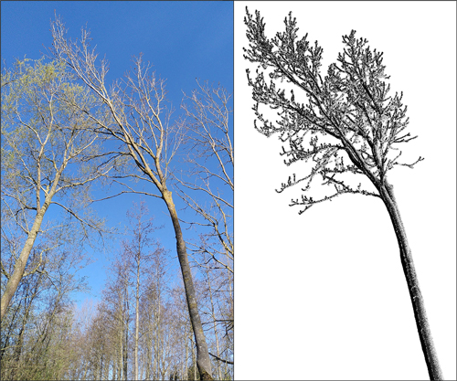
Fig. 1. Photograph and point cloud of common ash #2. (left) Ash #2 before felling (on the foreground). (right) Point cloud visualisation of the same tree from the same upward looking perspective as the photographer.
2.2 Terrestrial laser scanning
In total, 21 scans were acquired with a RIEGL VZ-400i laser scanner (RIEGL Laser Measurement Systems GmbH). This time-of-flight instrument has an exit beam diameter of 7 mm and a beam divergence of 0.35 mrad; at 25 m distance from the scanner this results in a Gaussian beam spot size of 16.75 mm. Scanning was performed at 300 kHz pulse repetition rate and 0.04° angular resolution; at every position a 360 degree panorama was captured between a zenith range of 30°–130°. To ensure capture of a full hemisphere, Wilkes et al. (2017) advise to combine an upright and tilted scan per position; however, a tilted scan was not performed here in order to better separate the impacts of the different positions.
A regular 10 m × 10 m grid with total dimensions of 40 m × 40 m covering 21 positions in total was laid out (Fig. 2); the two trees were located in the centre of the scanning domain. Although the grid-wise procedure is usually reserved for plot-level scanning rather than individual tree scans (Wilkes et al. 2017) it was used here to mimic the point cloud properties as if one was interested in all the trees in the forest plot. In total, 35 reflective targets on 180 cm long poles were randomly distributed inside the scanning area to facilitate coarse coregistration of individual scan positions. Additionally, a small reflective marker was attached exactly at breast height (130 cm) on the stems to retrieve the exact location of breast height for DBH measurements in the point clouds. Scans were acquired on 19/03/2020 in leaf-off conditions. During the scanning, there was no precipitation and the above-canopy wind speed forecast was 5–10 km h–1 or less. No movement of the upper branches could be observed from the ground.
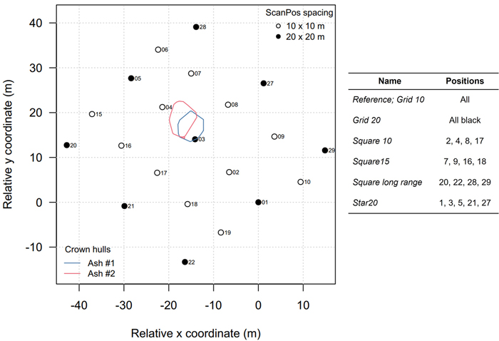
Fig. 2. Map of the scanning pattern. The locations of the harvested ash trees are depicted as vertical projections of their crown hulls. The scan positions of the modulations are shown on the right.
Coregistration is a two-step process involving a coarse and fine registration. Scans were coarsely registered using the reflective targets. Fine registration was then initially achieved using Multi-Station Adjustment 1 algorithm (MSA1) in the scanner manufacturer’s RiSCAN PRO 2.11.3 software. MSA1 iteratively aligns scans based on the minimisation of the distance between overlapping detected planar surfaces in adjacent scans.
The two target trees were manually segmented from the coregistered forest point cloud scene using CloudCompare. Next, noise points were filtered based on RIEGL VZ-series scanners specific point attributes: all points with a pulse shape deviation larger than 12 or a reflectance lower than –17 dB were removed (Calders et al. 2017). The pulse shape deviation attribute was used to remove points that could be originating from merged echo pulses from multiple intersected surfaces. The reflectance attribute, a measure for the ratio of the emitted vs. backscattered laser pulse power, was used to filter noise points with very low backscattered energy. The ranging distance (R) in meters was calculated as the Euclidean 3D distance between each point coordinate and its respective scan position origin.
2.3 Diameter reference measurements
After scanning, the two trees of interest were felled. For this, the forest floor was cleared to create a clean surface in the felling direction. Ash trees are known for their stiffness and are an excellent species to destructively assess branching architecture. The trees had little to no broken branches after felling impact which allowed to reconstruct the branching architecture on the ground and draw a branching topology of all the branches with a diameter (d) > 2.5 cm. Next, the branch dimensions were measured. For branch diameters d where d > 2.5 cm we used measuring tape with 0.5 mm readings to measure the circumference which was converted to d assuming a circular cross-section. For measurements where d < 2.5 cm the mean of two perpendicular measurements of d from 0.01 mm precision calipers was used. We cut and put aside all the branches where they tapered to d < 2.5 cm. Then, the stem was identified all the way up to the tree tip by following the largest branch at each bifurcation. The stem was marked every 80 cm with lumber crayon and the circumference over bark was measured. The locations where branches tapered exactly to d = {5, 7, 10 cm} were marked with coloured lumber crayon. All branches bifurcating from the stem were labelled A, B, C… starting from the lowest branch. For every branch we recorded i) the height along the stem where this branch was sprouting, ii) the total length of the branch (till taper of 2.5 cm diameter) and the length along the branch where the taper was 10 cm, 7 cm, or 5 cm, and iii) the diameter of the branch 10 cm after the bifurcation. For all branches of the second order and higher, the same procedure and measurements were followed (now codified as AA, AB, AC,…).
This resulted in three types of Location Of diameter Measurements (LOM):
- 10 cm from the base of the branch (TYPE 1)
- At d = {2.5, 5, 7, 10 cm} (TYPE 2)
- Every 80 cm along the stem (TYPE 3)
2.4 Destructive measurements of tree mass, density, and water content
After all branch length and diameter measurements were performed, we clipped and sawed the entire tree into five diameter classes: d = {<2.5, 2.5–5 cm, 5–7 cm, 7–10 cm, >10 cm}. Fresh weights were recorded with a top-loading balance (Kern & Sohn GmbH, Balingen, capacity 6000 g, precision 1 g) for the material with d < 10 cm, while for the larger material we used a tree suspended Dynafor LLX1 dynamometer (capacity 1000 kg, precision 0.5 kg), and weights were lifted with a hoist. The stump was weighed with the larger material. From each diameter class we took samples to assess wood basic density and dry matter content. In each of the smaller classes we randomly sliced five approximately 10 cm long branch pieces (five times a composite sample of five pieces in the d < 2.5 cm class). For the class d > 10 cm we sliced a 5 cm thick cross-sectional disc every 80 cm along the stem. An additional disc just above the stump (at 50 and 40 cm height respectively for ash #1 and #2) and at breast height (130 cm) were sampled as well. Chainsaw cuts were as much as possible performed after weighing to minimize the weight loss of the sawdust. The samples were cleaned with a brush (mostly to remove lichens in the upper part of the canopy) and weighed as fast as possible using the 6000 g capacity balance to determine the fresh mass (massfresh) to avoid water loss from the green wood samples. The time between felling and weighing was about four hours. We labelled the wood samples, packed them in plastic bags, and sealed the bags. On the same day, but after transportation to an indoor working environment (<12 h), the volume (Vfresh) of all the samples was measured using the Archimedes water displacement method. For this, we used the same 6000 g balance as before and submerged the samples in a container with water of ~15 ℃. For larger samples we used a 16 000 g/ 1 g precision balance. Weight readings were converted to volume assuming a density of 1000 g/L of the liquid. All samples were transferred to a drying stove at 103 ℃ and dried until the largest sample was at constant weight (less than 1 g change over 24 h) + an extra of 48 h. Then, the dry mass (massdry) was weighed. We calculated the dry matter content (DMC), fresh wood density (FWD) and basic wood density (ρ) of each sample or composite sample as:
DMC = massdry / massfresh (%), and
FWD = massfresh / Vfresh (kg m–3), and
ρ = massdry / Vfresh (kg m–3)
The DMC, FWD and ρ of each diameter class for each tree was estimated by summing the mass or volumes of the samples in each class and then calculating the ratio as above, except for the diameter class >10 cm. For this class, we weighted the DMC, FWD and ρ of each disc by its cross-sectional area (Demol et al. 2021). The destructively assessed fresh weight was converted to biomass and fresh volume through multiplication by DMC and division by FWD, respectively.
2.5 Locating the manual diameter measurements in the point cloud
The LOM were traced back on point clouds of the individual trees using the branching topology. A segment of 10 cm length was extracted from the point cloud around each LOM using CloudCompare. To find the centre of each 10 cm long branch segment, a cylinder was fitted to these branch segment point clouds using the M-estimator SAmple Consensus (MSAC) algorithm with a maximum inlier-cylinder distance of 1 mm, which is implemented in Matlab’s pcfitcylinder function. The centre point P of the cylinder’s axis was extracted. An arbitrary yet conservative threshold was used to detect obviously erroneous cylinder fits: in case the diameter of the fitted cylinder exceeded 1.5 times the diameter of the manual measurements, we instead used the centroid of the point cloud segment itself for P. This was needed for branch segment point clouds with only a few or linearly arranged points and hence where a cylinder fit was not appropriate.
2.6 Point cloud modulations
We applied two types of subsetting procedures to make several ‘versions’ of the single tree point clouds – called modulations (Table 2). On one hand, we created point clouds by only including points from certain scan positions (Fig. 3). This mimicked popular dedicated scan patterns that are mainly used in single tree TLS data acquisition campaigns (Wilkes et al. 2017). In total, five scan pattern modulations were constructed in square or star-like configurations with varying sizes, apart from the 10 × 10 m grid reference (all scan positions, called ‘Grid 10’). On the other hand, we applied a range filter procedure by only including the points that had a range R closer than a threshold value. A shorter range implies, ceteris paribus, a smaller beam spot size and hence a reduced uncertainty in the measurement. We selected the following thresholds: R < {20, 22.5, 25, 30, 35}. Point clouds with maximum ranges lower than 20 m were partly occluded and resulted in erroneous volume models, hence we started with 20 m as the lowest R filter threshold. The range filters were applied to the scan position modulation ‘Grid 10’ that included all the 21 scan positions. Next, all point cloud modulations were downsampled to only keep maximum one point per 1 mm voxel.
| Table 2. The 14 point cloud modulations constructed for each of the two ash trees. | ||
| Modulation type | Name | Description |
| Reference | Grid 10 | 10 × 10 m square grid, MSA1, filtered for deviation and reflectance |
| Scan pattern | Grid 20 Square 10 Square 15 Square longrange Star | See Fig. 3 and text |
| Range | Range20 … Range 35 | Points further away than respectively 20, 22.5, 25, 30, 35 m removed |
| Unfiltered | Unfiltered | Same as Reference but without filtering |
| Fuzz filtering | Fuzz | Same as Reference but with additional Fuzz filtering |
| Multi-station adjustment module 2 | MSA2 | Same as Reference but MSA 2 instead of MSA1 |
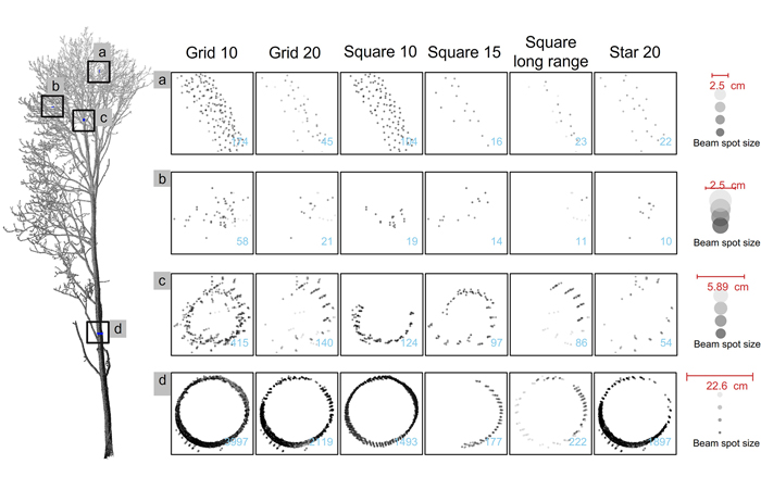
Fig. 3. Examples of common ash branch segment point clouds under a variation of scan position layouts. See Fig. 2 for a description of scan position variations. Segments have a zenith point of view. Points coloured on beam spot size; red bar shows the true-to-scale manually measured branch diameters at each location and the true-to-scale beam spot sizes. In blue the number of points per segment is shown. The manual diameters were 25, 25, 58.9, and 226 mm each segment. View larger in new window/tab.
2.7 Reflectance ‘fuzz’ filter and improved coregistration
We tested two error mitigation strategies. The first is a reflectance filtering procedure to remove scattered points as designed by Wilkes et al. (2021) which we will call the ‘fuzz’ filter. Scattered points are points where the beam footprint intersects the surface of the scanned objects and triggers a return, yet, without the centroid of the emitted laser beam intersecting the object. Locally around individual branches in the point cloud, the expected minimum reflectance could be modelled from the observed maximum reflectance. All points with a reflectance lower than the expected reflectance, multiplied with a threshold value of 0.8, were removed. This procedure was implemented in a voxelised point cloud (dimensions 50 × 50 × 50 mm) and for each individual scan position separately, as reflectance characteristics vary locally depending on e.g. branch size, distance to the scanner, the orientation of the beam respective of the branch surface. Finally, a nearest neighbour filter was used to delete isolated points. Isolated points had a distance to the 10 closest neighbours (dNN10) that was larger than the mean + standard deviation of the dNN10 of the whole point cloud. A detailed description and theoretical background can be found in Wilkes et al. (2021). For an example of a filtered point cloud, see Supplementary file S1. The fuzz filter was applied to the full ‘Grid 10’ modulation.
The second tested mitigation strategy is the automated and improved algorithm Multi-Station Adjustment 2 (MSA2) used for finely registering individual scans to a common coordinate system. Using MSA1 we obtained visually good coregistration results of the trunk and main branches yet finely aligning branches was beyond the capabilities of MSA1. MSA2 differs from MSA1 because it uses additional information of an inertial measurement unit (IMU) and real-time kinematic corrected GNSS positioning in coregistering scans. Similar to MSA1, proximate planar surfaces in neighbouring scans are iteratively aligned, yet in MSA2 this process is almost entirely automated and requires only minimal user input. Additional details could not be disclosed by RIEGL (pers. comm. on March 24, 2021). In total, this resulted in 14 modulated point clouds per tree; the Grid 10 reference cloud, five from scan pattern modulation, five from range modulation, one unfiltered modulation, one modulation from fuzz filtering, and one from MSA2 implementation.
2.8 QSM reconstructions
For each of the 14 point cloud modulations, 3D cylindrical reconstructions of tree aboveground volume were generated using TreeQSM v2.4.0 (https://github.com/InverseTampere/TreeQSM) (Fig. 4). In TreeQSM v2.4.0, the point cloud section where a cylinder is fitted, is first filtered for outliers using so-called surface coverage filtering. For this, a point cloud section is partitioned into cells (intersections of sectors and layers) based on their height and angle as seen from the estimated cylinder axis. There are 20 equal angle sectors and the height of the layers and the cells is 2 cm. For each cell only the points closest to the axis are kept.
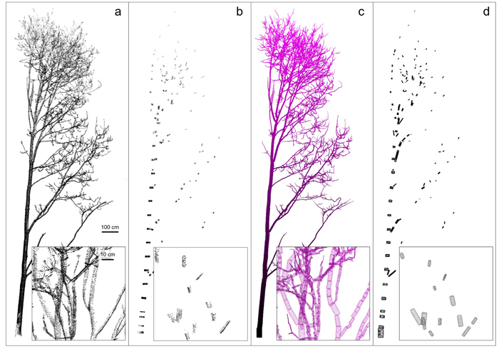
Fig. 4. TLS point cloud and QSM reconstruction of common ash #2. Bottom: magnification of branches in the upper part of the crown (location indicated by the parallelogram – direction of view indicated by the arrow in panel c). (a) Full point cloud. (b) Manually segmented 10 cm long branch sections. (c) Full QSM of the tree (coloured by z-coordinate value). (d) Individual QSM cylinders that have been successfully matched with the manual measurements. View larger in new window/tab.
The ideal input parameters for TreeQSM depend on, among others, the point cloud density, data acquisition conditions, and foliage of trees of interest. Therefore, the models were run: a) for a suite of realistic input parameters, and b) for five iterations per unique input parameter combination (replicates). For our point clouds, the resulting total QSM volume was most sensitive to the parameter PatchDiam2Min, and to a lesser extent to PatchDiam2Max. PatchDiam2Min controls the minimum size of patches into which the tree surface is partitioned at the branch tips. Smaller patches can better resolve smaller branching elements but come at a computational cost and too small values can lead to over-segmentation, i.e., segmenting a branch into two or more segments. Similarly, PatchDiam2Max controls the maximum patch size at the bottom of the tree. Further details can be found in the TreeQSM documentation; see also Gonzalez de Tanago et al. (2018). We kept all other input parameters constant and ran TreeQSM with a range of PatchDiam2Min and PatchDiam2Max values, resulting in 28 unique input parameter combinations per modulation per tree. The input parameters were:
- PatchDiam1 = 150 mm
- PatchDiam2Min from 5 mm to 20 mm (in 2.5 mm steps)
- PatchDiam2Max: {15, 20, 30, 40 mm}
- Taper and parent correction to a minimum cylinder diameter of 2.5 mm
- Other parameters at default values
For each input parameter combination five replicate models were constructed. The optimal input parameter set per modulation was selected based on minimisation of the sum of the mean point-model distance of the trunk and branches of these five models. A visual check of point cloud-model overlays of the selected QSMs was used to select this criterion. We tested several other optimisation criteria, inter alia minimisation of the deviation on total and trunk volume for repeated runs, minimisation of the mean and maximum point-model distance, and maximisation of the surface coverage of cylinders by point cloud segments. However, these other criteria were not able to consistently produce the best models, especially for the sparser point clouds (e.g. the Range20 or Square10 modulations). Finally, from the five replicate models with optimal PatchDiam2Min – PatchDiam2Max combination, we retained the model with volume closest to the mean of five volumes for further analysis. We used the standard deviation of the volumes of the five replicates as measure of uncertainty of the reconstructions. In total, 3920 models were constructed: 5 replicates of 28 input parameter combinations run for 14 point cloud modulations for two trees.
2.9 Matching manual and QSM diameter measurements
We implemented a procedure to match the branch centroids P with the closest cylinder in a QSM reconstruction. For this, the distance between P (a 3D point in space) and the axes of all QSM cylinders (a 3D line segment) was calculated; the QSM cylinder with the closest distance to P was withheld. Any matches with d(P,QSM) > 5 cm were removed to ensure close agreement of the manual measurements with the 3D reconstructions.
Overall, this resulted in three types of diameter measurements per LOM: from manual circumference measurements (converted to diameters assuming circular branch cross-sections), from cylinder fitting of a 10 cm point cloud segments, and finally the diameter from the QSMreconstructions. The latter consisted of 14 diameters (one for each optimised modulation).
2.10 Statistical analysis
Differences between manual measurements and QSM-derived estimates of branch diameter were tested with a one-sided paired t-test after testing for normality with a Shapiro-Wilkes test. A non-parametrical Wilcoxon test was used when n < 40 for non-normally distributed differences.
3 Results
3.1 Volumetric comparison
The two ash trees had a destructively assessed fresh mass of 647 kg and 713 kg and an aboveground volume of 732 L and 868 L, respectively (Table 3). The wood properties FWD, DMC and ρ showed only minor variation with branch diameter category (less than 50 kg m–3 and 0.05 kg kg–1 difference respectively), except for the branches d < 2.5 cm which had lower values for FWD, DMC and ρ (respectively 36–75 kg m–3, 74–113 kg m–3 and 0.063–0.091 kg kg–1 less than the other categories). Within branch categories the standard deviation of FWD, DMC and ρ of five (composite) samples was generally small, and was maximum 54 kg m–3 (for FWD for the 5–7 cm class for ash #1) (Table 3).
| Table 3. General characteristics of the harvested common ash trees and overview of destructive tree mass measurements, conversion factors and converted volumes for two ash trees. The results are divided into diameter classes of the sampled material. ‘Full tree’ marks either the total mass or volume per tree, or the weighted wood properties. Additionally, the compartmentalised volumes of the optimised reference modulation quantitative structure model (QSM) are added. AGB: aboveground biomass. FWD: Fresh wood density. ρ: Basic wood density. DMC: dry matter content. We used ‘tree length’ rather than tree height because this was measured on the felled tree. | |||||||||||
| DBH (cm) | Tree length (cm) | Scan & harvest date | Fresh mass (kg) | Volume (L) | QSM (L) | AGB (kg) | FWD (kg m–3) | ρ (kg m–3) | DMC (kg kg–1) | ||
| Ash #1 | 27.4 | 1957 | 19/03 & 03/04 2020 | Full tree | 646.5 | 731.9 | 1114 | 421.4 | 883 | 576 | 0.652 |
| >10 cm | 456.5 | 506.7 | 542 | 300.5 | 901 | 593 | 0.658 | ||||
| 7–10 cm | 34.0 | 39.4 | 60.6 | 22.7 | 864 | 577 | 0.668 | ||||
| 5–7 cm | 44.9 | 53.4 | 61.8 | 30.2 | 841 | 565 | 0.672 | ||||
| 2.5–5 cm | 53.6 | 62.8 | 234 | 34.6 | 855 | 551 | 0.645 | ||||
| 0–2.5 cm | 57.4 | 69.5 | 216 | 33.4 | 826 | 480 | 0.581 | ||||
| Ash #2 | 29.4 | 1905 | 19/03 & 07/04 2020 | Full tree | 713.1 | 868.2 | 1201 | 461.0 | 821 | 531 | 0.647 |
| >10 cm | 509.0 | 620.6 | 643 | 332.8 | 820 | 536 | 0.654 | ||||
| 7–10 cm | 34.9 | 41.3 | 58.9 | 22.9 | 844 | 555 | 0.658 | ||||
| 5–7 cm | 34.3 | 40.8 | 67.4 | 22.5 | 840 | 551 | 0.655 | ||||
| 2.5–5 cm | 70.2 | 85.4 | 256 | 44.4 | 823 | 520 | 0.632 | ||||
| 0–2.5 cm | 64.7 | 80.0 | 176 | 38.5 | 808 | 481 | 0.595 | ||||
The optimal QSM model from the reference Grid 10 modulation had, for both trees, input parameters PatchDiam2Min = 0.75 cm and PatchDiam2Max = 2 cm. Lowering PatchDiam2Min values led to over-segmentation and ‘ivy’ like cylinder fits on the surface of the tree trunk (Suppl. file S2). The average (± standard deviation) total volume of five models from the reference modulation with the optimal input parameter combination was 1114 ± 9 L and 1201 ± 8 L (Table 3). This was considerably more than the destructively assessed tree volumes: the solid wood volume (all parts > 10 cm diameter) was overestimated by 6.3% and 3.2% for ash #1 and #2 respectively, while the total volume was overestimated by 52% and 38%.
The absolute difference with destructive volume measurements for the optimal model were the largest for d between 2.5 and 5 cm: here, we observed a surplus of 170 L for both trees (accounting for 45% and 51% of the total tree volume overestimation) (Table 3). The second to largest absolute differences were found in branches with d < 2.5 cm: these were overestimated by 146 L (ash #1) and 96 L (ash #2) and were as such responsible for 38% and 29% of the overestimation on whole-tree level volume (Fig. 5).
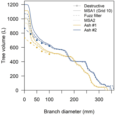
Fig. 5. QSM and destructive cumulative volume repartitioning in common ash based on branch diameter sizes. Grey/white bands indicate the branch diameter classes used in the destructive measurements. QSM volumes obtained with the Grid 10 modulation (coregistered using Multi-Station Adjustment 1 (MSA1)), a fuzz filtered and MSA2 point cloud.
3.2 Diameter comparisons
For QSMs with optimal input parameters, we were able to successfully locate all manually measured branch LOMs to the correct QSM cylinder. Generally, the diameter of smaller branches was overestimated by QSM reconstruction, and the relative diameter error increased with decreasing branch diameter (Fig. 6). For the Grid 10 modulation the diameters of parts > 10 cm were on average overestimated by +4% (two-sided paired t-test: p < 0.01). In contrast, for the branches d < 2.5 cm this overestimation was +73% (two-sided paired t-test: p < 0.01) (Table 3). The uncertainty of the QSM branch diameter estimates was assessed by computing the standard deviation of the diameters of 5 QSM iterations with identical input parameters for each scan modulation. In general, the absolute uncertainty remained constant across the diameter range meaning that the relative uncertainty increased towards the smallest branches (Fig. 6). A comparison of manual diameter measurements with Matlab’s pcfitCylinder displayed very similar patterns as the comparison with QSM diameters (Suppl. file. S3). On average, the smaller the branch, the higher the overestimation by pcfitCylinder. The volume repartitioning per branch diameter size was similar for both trees (Fig. 5).
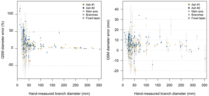
Fig. 6. Relative (left) and absolute (right) error in the diameter of common ash QSM cylinders from the reference point cloud ‘Grid 10’ with respect to manually measured branch diameters. Comparison of hand-measured branch diameters and diameters from five QSM reconstruction (mean and standard deviation as grey whiskers). Light-grey/white bands indicate branch diameter classes. The fixed taper measurements are located at the thresholds of the diameter classes. For reasons of clarity, here no standard deviation whiskers are plotted. For visualisation purposes one outlier (error = 257% and hand-measured diameter = 3.3 mm) is not within the plotting frame. View larger in new window/tab.
3.3 Scanning position modulation
We observed similar patterns of overestimation in the modulated point clouds as in the ‘Grid10’ reference scan (Fig. 7). Total volume was still overestimated – though the magnitude differed considerably between modulations (overestimations ranging approx. 150–550 L and 140–640 L for the two trees). These differences were more pronounced in the smaller branch categories. The branch categories d < 10 cm were overestimated across most modulations. The absolute difference was largest in category d = 2.5–5 cm. Range filtering was effective to reduce the overestimation in the 2.5–5 cm category and had little effect in the other categories (Fig. 7). For the ‘No filter’ modulation (Table 2), the overestimation was considerably increased (50–70% overestimation of the total tree volume). The modulation ‘Grid20’ produced QSMs with the largest overestimation: here, total tree QSM volume was 1350 L (ash #1) and 1349 L (ash #2) versus reference volumes of 732 L and 868 L, respectively (Fig. 7). The max range modulations had a modestly increasing overall volume when including points from further ranges. These differences mainly originated in the d = 2.5–5 cm category. Scanning layout modulation had mixed effects. Overall, the patterns that were used here resulted in two- to five-fold higher standard deviations on volumes of repeated model runs with respect to Grid10 (Fig. 7). The accuracy of tree volume was variable: the square-type layouts had an increasing overestimation for larger distances between positions.
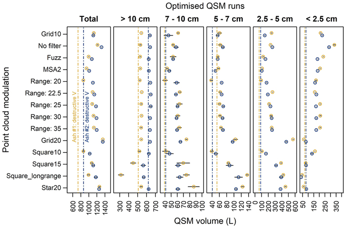
Fig. 7. Comparison of the QSM volume against destructively measured volume (dashed line) in 5 diameter classes for 12 different point cloud modulations, the fuzz filtered point cloud and the Multi-Station Adjustment 2 coregistration in two common ash trees. QSM volume was extracted as the mean (points) and standard deviation (black whiskers) of five models with optimal input parameters. See Fig. 2 for a description of the scanning patterns.
3.4 Reducing small branch overestimation with ‘Fuzz Filter’ and MSA2
The accuracy of the QSM diameters from a fuzz-filtered point cloud improved with respect to the original (non-filtered) point cloud (Fig. 5 and Fig. 8). However, in general there was still an increasing branch dimension overestimation towards the smaller branches. The solid volume (i.e. all parts d > 10 cm) was modestly overestimated by 4.3% (for reference: ash #1, 6.2% without fuzz filtering) and 1.4% (ash #2, 3.2% without fuzz filter). The diameters of fuzz filtered branches larger than 10 cm were modestly larger than the manual measurements (one-sided paired t-test: p < 0.05 for branch measurements of both trees) and there was weak evidence that they were smaller than the non-fuzz-filtered modulation (MSA1) (one-sided paired t-test: p < 0.1). Smaller branches, such as the branches with d = 2.5 cm, were slightly larger than the manually measured branches (one-sided paired t-test: p < 0.1). However, they were significantly smaller than the non-fuzz-filtered branches (one-sided paired t-test: p < 0.001). The total volume was still overestimated by 36% and 18% (compared with 52% and 38% without fuzz filter) (Fig. 7 and Suppl. file S4).
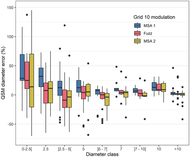
Fig. 8. Common ash branch diameter error of QSMs with respect to manually measured branches in branch diameter classes. Positive values indicate an overestimation of QSM diameters with respect to manual measurements. Three modulations were compared: the ‘Grid 10’ reference modulation using the standard Multi-Station Adjustment 1 (MSA1) algorithm, the fuzz filtered point cloud and the MSA2 registered point cloud. For visualisation purposes one outlier (error = 257% and diameter class <2.5 mm; MSA1) is not within the plotting frame. Box line represents median value, the upper and lower hinges represent the 25th and 75th percentile and the whiskers extend to the min/max values, except if min/max values are further than 1.5 times the interquartile range (these points are outliers: black dots).
The improved and automated MSA2 algorithm for finely aligning laser scans improved the accuracy of QSM-derived branch diameters and the overall tree volume with respect to the conventional alignment procedure (Fig. 5 and Fig. 8). Similar to fuzz filtering, these improvements occurred in all diameter classes yet were most pronounced in the diameter class d = 2.5 – 5 cm, with branch diameter considerably lower than MSA1 (one-sided paired t-test: p < 0.001). The overall volume was 944 and 1011 L for ash #1 and #2 respectively which represented an overestimation of 29% and 16%, while the solid wood was overestimated by 4.5% and 1.0% (Fig. 7, 8 and Suppl. file S4).
4 Discussion
4.1 TLS-derived tree volume is overestimated in smaller branches
Here, we presented the first branch diameter validation in leaf-off operational conditions for TLS-derived 3D tree reconstructions. The most important observation was an overestimation of the TLS-derived diameters of small branches (Fig. 6). The relative overestimation increased for smaller branches. Consequently, the total aboveground volume from laser scanning for these trees was considerably overestimated (38% to 52%) compared to the destructive measurements. Branches with d < 5 cm accounted for 80–83% of the total overestimation.
Previous in situ, ex situ and in silico tests had identified problems in retrieving accurate estimates of volume and diameters of small-sized branches (Hackenberg et al. 2015b; Lau et al. 2019; Abegg et al. 2020). This was largely confirmed in the current study, which featured 265 manually measured branch diameters. Whereas branch diameters were sometimes poorly reconstructed with QSMs, tree and branching structure was very accurately reconstructed (Fig. 4). With all tested modulations we were able to retrieve all 265 manually measured branch locations in the QSMs, meaning that there was very little to no occlusion. This contrasts with tropical and leaf-on tree constructions, where often small branches are not even detected (Momo Takoudjou et al. 2018). For instance, for tall tropical trees, Lau et al. (2018) were not able to reconstruct 55% of branches with d = 10–20 cm.
For both trees, branches with d > 10 cm were modelled well (Fig. 8) and volume only differed by 6.3% and 3.2%. The critical diameter class, with the largest absolute volume overestimation, was d = 2.5–5 cm. This was caused by an inflation of d = 2.5–5 cm branches, but also by a proportion of branches that were in reality d < 2.5 cm but that had been overestimated and as such ended up in a larger class.
To our knowledge, the TLS experiment in tall, tropical, leaf-on trees of Lau et al. (2018) is at present the only one comparing in situ manual diameter measurements (other than DBH) with 3D reconstructions. In that tropical study the diameters of 10 to 20 cm sized branches were overestimated by 40%. Larger branches on the contrary were underestimated, so that the overall coarse woody volume was underestimated with an overall error of only 3%. Branches smaller than 10 cm diameter were not included. In our study we were able to measure and match much smaller diameters (down to 3.3 mm). In none of the diameter classes an underestimation of tree volume was observed (Fig. 8), resulting in a net volume overestimation at the total tree level.
4.2 A broad range of input parameters result in close-to-optimal QSM reconstructions
Here, we found that total tree volume was most sensitive to PatchDiam2Min (also observed by Calders et al. 2015; Gonzalez de Tanago et al. 2018). However, while PatchDiam2Min had a considerable influence on the volumes of small branches, its effect on average point-model distance and the variance in volume of repeated runs was minimal. Parameter optimisation with these metrics should be carefully implemented, especially if no ground-truth information is available. Due to the high-quality, non-occluded point clouds, there is a relatively large input parameter space that produces precise QSMs, and accurate solid volumes, yet inaccurate branch wood volumes. For example, for the ‘Grid10’ modulation we obtained close-to-optimal (in terms of optimisation metric) models with input parameters ranging in PatchDiam2Min form 7.5 mm to 15 mm and PatchDiam2Max from 15 mm to 40 mm yet varying in total volume by >20%. Similarly, the modulated scans produced precise QSMs with satisfying optimisation metrics (Fig. 7).
Additionally, the direct comparison of cylinder fits to point cloud segments showed a trend of overestimated smaller branches (Suppl. file S3). These cylinder fits, which are independent from the QSM reconstruction or its parameters, show a similar pattern of overestimation as seen in QSMs. We therefore exclude suboptimal input parameters to TreeQSM as the primary cause of the observed overestimations.
4.3 Branch diameter overestimation due to misalignment
Our dataset does not allow to disentangle all the potential sources of branch diameter inflation (namely misalignment, scattering, sparse point clouds, and suboptimal QSM parameterisation) due to a limited sample size. Within misalignment errors we identified wind and coregistration error. Here, scans were acquired on an apparent windless day. The wind effect was very small to negligible in this study. Coregistration error is hard to assess quantitatively. Yet, we argue that the coregistration error is potentially larger for small branches. The MSA procedure for finely coregistering point clouds is based on minimising the distance between planar fits through point cloud sections. Tree trunks (and possibly the forest floor if understory is absent) have a higher point density and lower curvature than small branches, allowing more planar fits and closer matches. Notwithstanding having obtained very precise coregistration with MSA1, the newer MSA2 procedure in our case allowed further improved branch coregistration (Suppl. file S1). MSA2 is largely based on the same principles as MSA1, yet unfortunately full details of MSA2 were not disclosed by RIEGL.
In our study, we only used the scanner in an upright position, resulting in a blind spot above the scanner where no data is collected. While this was needed to be able to assess the alignment from different positions with respect to the range to the position, it is recommended to also acquire a tilted scan to obtain a hemispherical view at each scan location (Wilkes et al. 2017). The upright-only strategy did not result in occlusion for the full grid scan. However, if tilted scans would have been acquired, the minimum range for unoccluded point clouds (in e.g. the range modulations) could have been diminished.
Misalignment error scales with the amount of superimposed scan positions. A context-specific trade-off in the number of scan positions arises: too few scanning positions will result in occlusion, whilst too many might increase misalignment errors (Pitkänen et al. 2019). Additionally, the placement of positions is important too; to minimise occlusion, Abegg et al. (2017) and Wilkes et al. (2017) advise to use an evenly spaced scanning grid. Conceptually, if each scan is equally likely to be affected by wind and coregistration, the misalignment error in the assembled point cloud will increase linearly with additional scan positions, whereas occlusion will diminish asymptotically (Fig. 9). This phenomenon was observed in the range-modulated volume reconstructions: the point cloud needed to be sufficiently covered by positions to allow reconstruction. Additional points increased the variance and size of reconstructed small branches.
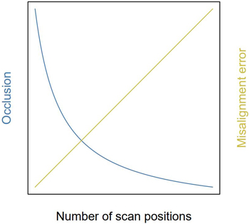
Fig. 9. Conceptual figure of the trade-off for optimal amount of scan positions. Theoretical implication of the number of scan positions on point cloud quality. This trade-off in amount of scan position balances the effects of occlusion and misalignment errors due to coregistration and wind.
4.4 Branch diameter overestimation due to scattering errors
Scattering errors are an important source of error around small branches that happen synchronously with alignment errors (Abegg et al. 2020). At the top of the canopy of a 20 m tall tree, the average beam spot size of the RIEGL VZ-400i is about 14 mm. This is almost on par with the average branch diameter at that height (Fig. 10). Additionally, tree crowns are complex environments where multiple non-planar, non-perpendicular objects intersect the laser beam path. This makes small branches highly susceptible to scattering errors, resulting in registered points outside of branches’ actual surface. This effect increases with either 1) smaller branches, or 2) larger intersecting beam spot sizes (which scale with distance from the scanner) (Abegg et al. 2021; Wilkes et al. 2021). For instance, the volume of branches d < 5 cm diameter was drastically increased when including points from further away scan positions while it did not affect the estimates of coarse woody volume (Fig. 7).
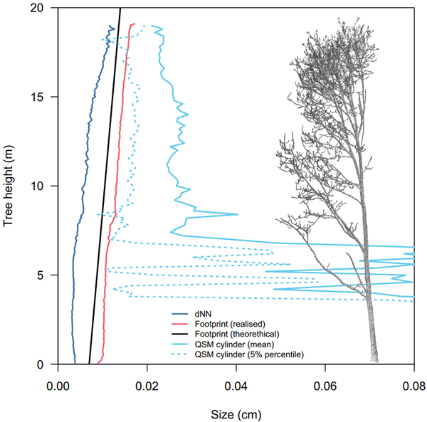
Fig. 10. Sizes of laser beam footprint, QSM cylinders and nearest neighbour distances of common ash #1 in function of tree height. dNN: the mean distance to the closest neighbouring point in 10 cm z-slices. The laser beam footprint diameter size was calculated from the ranging distance to the scanner. The realised footprint was inferred from the range of each point in the point cloud and averaged in 10 cm z-slices. The theoretical footprint was simulated from a scanner position at ground level. ‘QSM cylinder’ are the average and 5% percentile of QSM cylinder diameters in 20 cm z-slices.
The beam diameter and divergence are scanner specific (Table 1), yet it would be too simplistic to advise using a scanner with the smallest beam diameter possible. For instance, phase shift scanners typically have narrow beams yet are more susceptible to ranging noise from partial hits (Newnham et al. 2015). Larger footprints reconstruct the structure of the tree well as there is a reduced chance to miss small branches, exemplified by the 100% detection rate of the manually measured branches in the reconstructions. Additionally, time-of-flight instruments with multiple return detection capabilities are better suited to characterise complex environments like tree crowns (Wilkes et al. 2017).
4.5 Possible mitigation strategies to reduce branch inflation effects
The adverse effects of beam diameter size originate in a physical limitation in the scanner hardware, hence no easy fixes can be proposed to fully mitigate the small branch inflation observed in the current study. However, the fuzz filter approach sensu Wilkes et al. (2021) tested here was able to modestly reduce the small branch overestimation (Fig. 5). Its design specifically targets scattered points and will not correct for wind/coregistration effects. Misalignment in coregistration is a second important cause of branch overestimation, and will likely worsen the effects present in individual scans. A framework for objectively assessing coregistration accuracy in forest environments is currently lacking, and many algorithms are proprietary of the scanner manufacturer (but see e.g. Henning and Radtke (2008) and Liu et al. (2017) for alternative forest point cloud coregistration algorithms). Yet, here we showed that improving coregistration had a similar effect on QSM branch and volume accuracy as the fuzz filter. Using a max range filter with grid-wise scanning patterns is a straight-forward way of removing points originating from large beam footprint sizes. Similar future improvements might be obtained by moving the scanning position closer to the objects of interest with e.g. tall extendable tripods or drone mounted laser scanners (Brede et al. 2017). Another more complex possibility is to use each point’s estimated beam size as an additional uncertainty information for the diameter estimation. In this way each point would have different weight or uncertainty depending on its distance and the beam size and the points would not be equal in their contribution to the diameter estimation. Alternatively, returns could be represented as an ellipsoid that scales with uncertainty, instead of a discrete point in space. Other approaches use process-based or empirical predictions to overcome occlusion and sparse or low-quality point cloud sections in tree reconstructions (Côté et al. 2012; Hu et al. 2021).
Whereas the validation data for full-tree AGB estimates with TLS are increasing, little effort has been put into checking finer details such as branch diameters. We acknowledge that the number of trees and species is very limited in our study, yet the amount, precision and distribution of the manual diameter measurements form an important source of ground-truth data for developing/fine tuning novel filtering algorithms. However, it remains to be tested if other scanners or another forest environment will give similar results. For instance, ash trees seem to have an above-average volumetric proportion of small branches compared to other broadleaved European tree species (Longuetaud et al. 2013).
One issue has remained untouched thus far: why did earlier validation studies report remarkably more accurate volume estimates with TLS (Table 1)? We see three potential causes: either did the inflation of branches not happen, or it was balanced by an underestimation elsewhere, or the proportion of small branches was neglectable at the scale of the full tree/forest. If data was collected leaf-on, leaves occlude small branches (Calders et al. 2015; Gonzalez de Tanago et al. 2018). Leaf-stripping algorithms can be less or more conservative as to classifying leaf returns (Vicari et al. 2019; Krishna Moorthy et al. 2020a; Wang et al. 2020) yet many small branches are de facto removed if an additional leaf stripping algorithm was applied (Hackenberg et al. 2015a; Momo et al. 2020; Burt et al. 2021). Other authors did not take into account branches smaller than a certain diameter (e.g. Burt 2017).
Destructive harvest experiments are generally time-consuming and therefore often limited to a relatively small number of sampled trees (Table 1). It is critical to limit the uncertainties in fresh mass measurements and wood properties for conversion to AGB and woody volume (Demol et al. 2021). For this, we opted to limit the number of sampled trees in this work, but to measure them at a great level of detail (265 diameter and over 80 (composite) DMC, FWD and ρ measurements) with high-precision instruments. Here, potential systematic measurement errors were avoided by having independent measurements of tree mass (converted to volume with FWD) versus branch diameters. Although our study featured only two destructively harvested trees, it shows that above a certain branch diameter threshold, the effects of reflectance scattering and coregistration error are negligible. Abegg et al. (2020) for instance advise a 7 cm lower threshold based on a simulation study for beam diameter effects. In the present study, considering the best possible modulation (MSA2), this threshold could be lowered to 5 cm or even 2.5 cm. In future validation studies it is worthwhile to perform diameter measurements to assess this threshold.
5 Conclusion and outlook
In the eyes of the forest manager, the attractiveness of TLS roots in its capability to derive a 3D-explicit, traceable, and accurate snapshot of the forest in the form of point cloud. Through a diverse set of processing tools, a vast number of quantitative metrics can be extracted from point cloud data. Tree woody volume estimates from TLS are obtained with the reconstruction of entire trees as QSMs. Several potential sources of error are known to impact the accuracy of the TLS point cloud and/or the QSM reconstruction: misalignment, occlusion, scattering, and suboptimal QSM parameterisation. These errors and their interactions are poorly understood, the impacts on the estimation of tree metrics are largely unknown, and strategies to mitigate them are still under development.
Here, we showed that misalignment and scattering errors were the main cause of inaccuracies in QSM reconstructions of two Fraxinus excelsior trees. TLS-derived diameters of small branches (<10 cm) of leaf-off trees were generally larger than manually measured diameters. Smaller branches had larger relative errors. This resulted in an initial overestimation of tree woody volume. The magnitude of this overestimation (38–52%) was remarkably higher than other similar validation studies. We experimented with several strategies to improve the accuracy of branch diameter and tree woody volume estimates. In this work, it was demonstrated that the scan position layout, range filtering, coregistration precision, and filtering scattered points had variable but sometimes large effects on TLS-derived estimates of tree volume and branch diameter. The most effective strategy was a reflectance scattering filter procedure or an improved fine alignment of the point cloud that both halved the original overestimation. However, it was not possible to improve diameter estimates of branches with d < 2.5 cm. For future TLS forest inventories aiming at estimating tree volumes, we argue that the effect of beam divergence and beam spot size on point cloud quality should be carefully considered, as this is typically scanner model specific. Equally important is to minimise any misalignment errors (due to coregistration, or wind). The quality of the point cloud defines the lower diameter limit that still allows unbiased branch diameter estimates. Additional tests with different tree species, scanner types and reconstruction algorithms are needed to elucidate whether these conclusions can be generalised beyond our own study.
Authors’ contribution
MD: study design, data collection, data processing & Fig. preparation, writing: original draft. PW, PR: algorithm development, methodology, writing: review & editing. SMKM, KC: methodology, writing: review & editing. BG, HV: funding acquisition, writing: review & editing.
Acknowledgements
The authors want to thank Baldwin van Minnebruggen and Lisa De Wilde for last-minute covid-19 safe assistance with the field work. The harvested area was replanted with a mixture of Quercus robur L., Carpinus betulus L. and Betula pubescens Ehrh. on 02/03/2021.
Funding
MD was funded by the European Union’s Horizon 2020 research and innovation programme under grant agreement no 730944 - RINGO: Readiness of ICOS for Necessities of Integrated Global Observations. This study was supported by the ICOS Ecosystem Thematic Centre. PW was funded by the NERC National Centre for Earth Observation (NCEO). PR was funded by 3DForMod project of European Union’s Horizon 2020 research and innovation program ERA-NET FACCE ERA-GAS (ANR-17-EGAS-0002-01). HV and SMKM were funded by BELSPO (Belgian Science Policy Office) in the frame of the STEREO III programme – project 3D-FOREST (SR/02/355). KC was funded by the European Union’s Horizon 2020 research and innovation programme under the Marie Skłodowska-Curie grant agreement No 835398. BG was funded by Research Foundation Flanders (FWO) in the frame of ICOS infrastructure.
References
Abegg M, Kükenbrink D, Zell J, Schaepman ME, Morsdorf F (2017) Terrestrial laser scanning for forest inventories-tree diameter distribution and scanner location impact on occlusion. Forests 8, article id 184. https://doi.org/10.3390/f8060184.
Abegg M, Boesch R, Schaepman ME, Morsdorf F (2020) Impact of beam diameter and scanning approach on point cloud quality of terrestrial laser scanning in forests. IEEE Trans Geosci Remote Sens 59: 8153–8167. https://doi.org/10.1109/TGRS.2020.3037763.
Bienert A, Hess C, Maas HG, Von Oheimb G (2014) A voxel-based technique to estimate the volume of trees from terrestrial laser scanner data. Int Arch Photogramm Remote Sens Spat Inf Sci 40: 101–106. https://doi.org/10.5194/isprsarchives-XL-5-101-2014.
Brede B, Lau A, Bartholomeus HM, Kooistra L (2017) Comparing RIEGL RiCOPTER UAV LiDAR derived canopy height and DBH with terrestrial LiDAR. Sensors 17, article id 2371. https://doi.org/10.3390/s17102371.
Burt A, Boni Vicari M, da Costa ACL, Coughlin I, Meir P, Rowland L, Disney M (2021) New insights into large tropical tree mass and structure from direct harvest and terrestrial lidar. R Soc Open Sci 8, article id 201458. https://doi.org/10.1098/rsos.201458.
Burt AP (2017) New 3D measurements of forest structure. PhD Thesis, University College London.
Calders K, Newnham G, Burt A, Murphy S, Raumonen P, Herold M, Culvenor D, Avitabile V, Disney M, Armston J, Kaasalainen M (2015) Nondestructive estimates of above-ground biomass using terrestrial laser scanning. Methods Ecol Evol 6: 198–208. https://doi.org/10.1111/2041-210X.12301.
Calders K, Disney MI, Armston J, Burt A, Brede B, Origo N, Muir J, Nightingale J (2017) Evaluation of the range accuracy and the radiometric calibration of multiple terrestrial laser scanning instruments for data interoperability. IEEE Trans Geosci Remote Sens 55: 2716–2724. https://doi.org/10.1109/TGRS.2017.2652721.
Calders K, Adams J, Armston J, Bartholomeus H, Bauwens S, Bentley LP, Chave J, Danson FM, Demol M, Disney M, Gaulton R, Krishna Moorthy SM, Levick SR, Saarinen N, Schaaf C, Stovall A, Terryn L, Wilkes P, Verbeeck H (2020) Terrestrial laser scanning in forest ecology: expanding the horizon. Remote Sens Environ 251, article id 112102. https://doi.org/10.1016/j.rse.2020.112102.
Côté J-F, Fournier RA, Frazer GW, Olaf Niemann K (2012) A fine-scale architectural model of trees to enhance LiDAR-derived measurements of forest canopy structure. Agric For Meteorol 166–167: 72–85. https://doi.org/10.1016/j.agrformet.2012.06.007.
Côté J-F, Luther JE, Lenz P, Fournier RA, van Lier OR (2021) Assessing the impact of fine-scale structure on predicting wood fibre attributes of boreal conifer trees and forest plots. For Ecol Manage 479, article id 118624. https://doi.org/10.1016/j.foreco.2020.118624.
Dassot M, Colin A, Santenoise P, Fournier M, Constant T (2012) Terrestrial laser scanning for measuring the solid wood volume, including branches, of adult standing trees in the forest environment. Comput Electron Agric 89: 86–93. https://doi.org/10.1016/j.compag.2012.08.005.
Demol M, Calders K, Krishna Moorthy SM, Van den Bulcke J, Verbeeck H, Gielen B (2021) Consequences of vertical basic wood density variation on the estimation of aboveground biomass with terrestrial laser scanning. Trees 35: 671–684. https://doi.org/10.1007/s00468-020-02067-7.
Du S, Lindenbergh R, Ledoux H, Stoter J, Nan L (2019) AdTree: accurate, detailed and automatic modelling of laser-scanned trees. Remote Sens 11, article id 2074. https://doi.org/10.3390/rs11182074.
Faro Technologies Inc. (2009) FARO® Laser Scanner Photon 120/20 data sheet.
Gonzalez de Tanago J, Lau A, Bartholomeus H, Herold M, Avitabile V, Raumonen P, Martius C, Goodman RC, Disney M, Manuri S, Burt A, Calders K (2018) Estimation of above-ground biomass of large tropical trees with terrestrial LiDAR. Methods Ecol Evol 9: 223–234. https://doi.org/10.1111/2041-210X.12904.
Hackenberg J, Spiecker H, Calders K, Disney M, Raumonen P (2015a) SimpleTree – an efficient open source tool to build tree models from TLS clouds. Forests 6: 4245–4294. https://doi.org/10.3390/f6114245.
Hackenberg J, Wassenberg M, Spiecker H, Sun D (2015b) Non destructive method for biomass prediction combining TLS derived tree volume and wood density. Forests 6: 1274–1300. https://doi.org/10.3390/f6041274.
Henning JG, Radtke PJ (2008) Multiview range-image registration for forested scenes using explicitly-matched tie points estimated from natural surfaces. ISPRS J Photogramm Remote Sens 63: 68–83. https://doi.org/10.1016/j.isprsjprs.2007.07.006.
Hu M, Pitkänen TP, Minunno F, Tian X, Lehtonen A, Mäkelä A (2021) A new method to estimate branch biomass from terrestrial laser scanning data by bridging tree structure models. Ann Bot 128: 737–752. https://doi.org/10.1093/aob/mcab037.
Jackson T, Shenkin A, Wellpott A, Calders K, Origo N, Disney M, Burt A, Raumonen P, Gardiner B, Herold M, Fourcaud T, Malhi Y (2019) Finite element analysis of trees in the wind based on terrestrial laser scanning data. Agric For Meteorol 265: 137–144. https://doi.org/10.1016/j.agrformet.2018.11.014.
Krishna Moorthy SM, Calders K, Vicari MB, Verbeeck H (2020a) Improved supervised learning-based approach for leaf and wood classification from LiDAR point clouds of forests. IEEE Trans Geosci Remote Sens 5: 3057–3070. https://doi.org/10.1109/TGRS.2019.2947198.
Krishna Moorthy SM, Raumonen P, Van den Bulcke J, Calders K, Verbeeck H (2020b) Terrestrial laser scanning for non-destructive estimates of liana stem biomass. For Ecol Manage 456, article id 117751. https://doi.org/10.1016/j.foreco.2019.117751.
Kunz M, Hess C, Raumonen P, Bienert A, Hackenberg J, Maas HG, Härdtle W, Fichtner A, Von Oheimb G (2017) Comparison of wood volume estimates of young trees from terrestrial laser scan data. IForest 10: 451–458. https://doi.org/10.3832/ifor2151-010.
Lau A, Bentley LP, Martius C, Shenkin A, Bartholomeus H, Raumonen P, Malhi Y, Jackson T, Herold M (2018) Quantifying branch architecture of tropical trees using terrestrial LiDAR and 3D modelling. Trees 32: 1219–1231. https://doi.org/10.1007/s00468-018-1704-1.
Lau A, Calders K, Bartholomeus H, Martius C, Raumonen P, Herold M, Vicari M, Sukhdeo H, Singh J, Goodman RC (2019) Tree biomass equations from terrestrial LiDAR: a case study in Guyana. Forests 10, article id 527. https://doi.org/10.3390/f10060527.
Lehnebach R, Beyer R, Letort V, Heuret P (2018) The pipe model theory half a century on: a review. Ann Bot 121: 773–795. https://doi.org/10.1093/aob/mcx194.
Liu J, Liang X, Hyyppä J, Yu X, Lehtomäki M, Pyörälä J, Zhu L, Wang Y, Chen R (2017) Automated matching of multiple terrestrial laser scans for stem mapping without the use of artificial references. Int J Appl Earth Obs Geoinf 56: 13–23. https://doi.org/10.1016/j.jag.2016.11.003.
Longuetaud F, Santenoise P, Mothe F, Senga Kiessé T, Rivoire M, Saint-André L, Ognouabi N, Deleuze C (2013) Modeling volume expansion factors for temperate tree species in France. For Ecol Manage 292: 111–121. https://doi.org/10.1016/j.foreco.2012.12.023.
Momo Takoudjou S, Ploton P, Sonké B, Hackenberg J, Griffon S, de Coligny F, Kamdem NG, Libalah M, Mofack GI, Le Moguédec G, Pélissier R, Barbier N (2017) Using terrestrial laser scanning data to estimate large tropical trees biomass and calibrate allometric models: a comparison with traditional destructive approach. Methods Ecol Evol 9: 905–916. https://doi.org/10.1111/2041-210X.12933.
Momo Takoudjou S, Ploton P, Martin-Ducup O, Lehnebach R, Fortunel C, Sagang LBT, Boyemba F, Couteron P, Fayolle A, Libalah M, Loumeto J, Medjibe V, Ngomanda A, Obiang D, Pélissier R, Rossi V, Yongo O, Bocko Y, Fonton N, Kamdem N, Katembo J, Kondaoule HJ, Maïdou HM, Mankou G, Mbasi M, Mengui T, Mofack GII, Moundounga C, Moundounga Q, Nguimbous L, Ncham NN, Asue FOM, Senguela YP, Viard L, Zapfack L, Sonké B, Barbier N (2020) Leveraging signatures of plant functional strategies in wood density profiles of African trees to correct mass estimations from terrestrial laser data. Sci Rep 10, article id 2001. https://doi.org/10.1038/s41598-020-58733-w.
Newnham GJ, Armston JD, Calders K, Disney MI, Lovell JL, Schaaf CB, Strahler AH, Danson FM (2015) Terrestrial laser scanning for plot-scale forest measurement. Curr For Reports 1: 239–251. https://doi.org/10.1007/s40725-015-0025-5.
Pitkänen TP, Raumonen P, Kangas A (2019) Measuring stem diameters with TLS in boreal forests by complementary fitting procedure. ISPRS J Photogramm Remote Sens 147: 294–306. https://doi.org/10.1016/j.isprsjprs.2018.11.027.
Pyörälä J, Liang X, Vastaranta M, Saarinen N, Kankare V, Wang Y, Holopainen M, Hyyppä J (2018) Quantitative assessment of scots pine (Pinus Sylvestris L.) whorl structure in a forest environment using terrestrial laser scanning. IEEE J Sel Top Appl Earth Obs Remote Sens 11: 3598–3607. https://doi.org/10.1109/JSTARS.2018.2819598.
Pyörälä J, Kankare V, Liang X, Saarinen N, Rikala J, Kivinen VP, Sipi M, Holopainen M, Hyyppä J, Vastaranta M (2019) Assessing log geometry and wood quality in standing timber using terrestrial laser-scanning point clouds. Forestry 92: 177–187. https://doi.org/10.1093/forestry/cpy044.
RIEGL Laser Measurement Systems GmbH (2020) RIEGL VZ ®-400i data hheet.
Raumonen P, Kaasalainen M, Åkerblom M, Kaasalainen S, Kaartinen H, Vastaranta M, Holopainen M, Disney M, Lewis P (2013) Fast automatic precision tree models from terrestrial laser scanner data. Remote Sens 5: 491–520. https://doi.org/10.3390/rs5020491.
Trochta J, Král K, Janík D, Adam D (2013) Arrangement of terrestrial laser scanner positions for area-wide stem mapping of natural forests. Can J For Res 43: 355–363. https://doi.org/10.1139/cjfr-2012-0347.
Trochta J, Kruček M, Vrška T, Kraâl K (2017) 3D Forest: an application for descriptions of three-dimensional forest structures using terrestrial LiDAR. PLoS One 12, article id e0176871. https://doi.org/10.1371/journal.pone.0176871.
Vaaja MT, Virtanen J-P, Kurkela M, Lehtola V, Hyyppä J, Hyyppä H (2016) The effect of wind on tree stem parameter estimation using terrestrial laser scanning. ISPRS Ann Photogramm Remote Sens Spat Inf Sci III–8: 117–122. https://doi.org/10.5194/isprsannals-iii-8-117-2016.
Van Den Berge S, Vangansbeke P, Calders K, Vanneste T, Baeten L, Verbeeck H, Krishna Moorthy SP, Verheyen K (2021) Biomass expansion factors for hedgerow-grown trees derived from terrestrial LiDAR. BioEnergy Res 14: 561–574. https://doi.org/10.1007/s12155-021-10250-y.
Van Langenhove L, Depaepe T, Verryckt LT, Fuchslueger L, Donald J, Leroy C, Krishna Moorthy SM, Gargallo-Garriga A, Ellwood MDF, Verbeeck H, Van Der Straeten D, Peñuelas J, Janssens IA (2021) Comparable canopy and soil free-living nitrogen fixation rates in a lowland tropical forest. Sci Total Environ 754, article id 142202. https://doi.org/10.1016/j.scitotenv.2020.142202
Ver Planck NR, MacFarlane DW (2014) Modelling vertical allocation of tree stem and branch volume for hardwoods. Forestry 87: 459–469. https://doi.org/10.1093/forestry/cpu007.
Vicari MB, Disney M, Wilkes P, Burt A, Calders K, Woodgate W (2019) Leaf and wood classification framework for terrestrial LiDAR point clouds. Methods Ecol Evol 10: 680–694. https://doi.org/10.1111/2041-210X.13144.
Wang D, Momo Takoudjou S, Casella E (2020) LeWoS: a universal leaf-wood classification method to facilitate the 3D modelling of large tropical trees using terrestrial LiDAR. Methods Ecol Evol 11: 376–389. https://doi.org/10.1111/2041-210X.13342.
Wilkes P, Lau A, Disney M, Calders K, Burt A, Gonzalez de Tanago J, Bartholomeus H, Brede B, Herold M (2017) Data acquisition considerations for terrestrial laser scanning of forest plots. Remote Sens Environ 196: 140–153. https://doi.org/10.1016/j.rse.2017.04.030.
Wilkes P, Shenkin A, Disney M, Malhi Y, Bentley LP, Vicari MB (2021) Terrestrial laser scanning to reconstruct branch architecture from harvested branches. Methods Ecol Evol 12: 2487–2500. https://doi.org/10.1111/2041-210X.13709.
Total of 47 references.
