Jussi Manner  ,
Lauri Palmroth,
Tomas Nordfjell,
Ola Lindroos
,
Lauri Palmroth,
Tomas Nordfjell,
Ola Lindroos
Load level forwarding work element analysis based on automatic follow-up data
Manner J., Palmroth L., Nordfjell T., Lindroos O. (2016). Load level forwarding work element analysis based on automatic follow-up data. Silva Fennica vol. 50 no. 3 article id 1546. https://doi.org/10.14214/sf.1546
Highlights
- Recent developments in on-board technology enables automatic collection of follow-up data on forwarder work
- Time consumption per load was more strongly associated with Loading drive distance than with extraction distance, indicating that the relevance of extraction distance as a main indicator of forwarding productivity should be re-considered
- Data, within variables, were positively skewed with a few exceptions with normal distributions.
Abstract
Recent developments in on-board technology have enabled automatic collection of follow-up data on forwarder work. The objective of this study was to exploit this possibility to obtain highly representative information on time consumption of specific work elements (including overlapping crane work and driving), with one load as unit of observation, for large forwarders in final felling operations. The data used were collected by the John Deere TimberLink system as nine operators forwarded 8868 loads, in total, at sites in mid-Sweden. Load-sizes were not available. For the average and median extraction distances (219 and 174 m, respectively), Loading, Unloading, Driving empty, Driving loaded and Other time effective work (PM) accounted for ca. 45, 19, 8.5, 7.5 and 14% of total forwarding time consumption, respectively. The average and median total time consumptions were 45.8 and 42.1 minutes/load, respectively. The developed models explained large proportions of the variation of time consumption for the work elements Driving empty and Driving loaded, but minor proportions for the work elements Loading and Unloading. Based on the means, the crane was used during 74.8% of Loading PM time, the driving speed was nonzero during 31.9% of the Loading PM time, and Simultaneous crane work and driving occurred during 6.7% of the Loading PM time. Time consumption per load was more strongly associated with Loading drive distance than with extraction distance, indicating that the relevance of extraction distance as a main indicator of forwarding productivity should be re-considered.
Keywords
harvesting;
cut-to-length logging;
haulage;
data gathering;
automatic recording;
classification algorithm;
Hidden Markov Models
-
Manner,
The Forestry Research Institute of Sweden (Skogforsk), Uppsala Science Park, SE-751 83 Uppsala, Sweden
E-mail
jussi.manner@skogforsk.se
- Palmroth, John Deere Forestry, P.O. Box 472, FI-33101 Tampere, Finland E-mail PalmrothLauri@JohnDeere.com
- Nordfjell, Swedish University of Agricultural Sciences, Department of Forest Biomaterials and Technology, SE-901 83 Umeå, Sweden E-mail tomas.nordfjell@slu.se
- Lindroos, Swedish University of Agricultural Sciences, Department of Forest Biomaterials and Technology, SE-901 83 Umeå, Sweden E-mail ola.lindroos@slu.se
Received 7 January 2016 Accepted 7 April 2016 Published 13 May 2016
Views 168119
Available at https://doi.org/10.14214/sf.1546 | Download PDF

1 Introduction
As previously noted, despite a 50-year history much remains unknown about forwarding work, relative to harvesting work (Manner et al. 2013). This is partly because forwarding work datasets often cover only a few complete work cycles, i.e. forwarded loads, while harvester work datasets compiled in similar timeframes cover large numbers of complete work cycles, i.e. harvesting single trees (see, e.g., Nurminen et al. 2006). Forwarding a load normally takes almost an hour, so collecting even relatively small forwarding work datasets takes a long time by traditional manual recording methods (see, e.g., Kellogg and Bettinger 1994; McNeel and Rutherford 1994; Gullberg 1995; Tufts 1997; Tiernan et al. 2004; Mederski 2006; Nurminen et al. 2006).
Another complication is that in work observation studies forwarding is generally divided into separate work elements, but the number and definitions of work elements can vary almost infinitely, as no generally acknowledged nomenclature is used (cf. Kuitto 1994; Andersson 2015). However, forwarding is usually divided into five work elements: 1) Driving empty, 2) Loading, 3) Loading drive, 4) Driving loaded and 5) Unloading (including unloading drive) (see, e.g., Bergstrand 1985; Väkevä et al. 2001; Nurminen et al. 2006). Moreover, as driving and crane work can occur simultaneously, successive work elements may overlap. However, to simplify work element determination, the overlaps of successive work elements can be ignored by applying a priority rule, e.g. by setting a tyre rotation alone, or crane movement alone, as the determinant of a change of work element (see, e.g., Tiernan et al. 2004). In addition to possible overlaps of work elements, several steering, driving and crane functions may be in use simultaneously, which further increases simultaneous activity. However, overlapping intervals have been separately recorded in few (if any) forwarding work observation studies. In contrast, in long-term follow-up studies forwarding time consumption is typically analysed as whole cycles, i.e. forwarding is not divided into work elements (see, e.g., Eriksson and Lindroos 2014).
Forwarding follow-up studies are usually based on records extracted from the forest companies’ own information systems (see, e.g., Holzleitner et al. 2011; Eriksson and Lindroos 2014). Such studies provide representative datasets, but their resolution and reliability are questionable as observations are partly reported by the operators themselves. In contrast, well documented time data on forwarding can be obtained from standardized experiments (see, e.g., Manner et al. 2013). Standardized experiments have the advantageous ability to isolate effects of specific variables, but they generally yield small datasets. Furthermore, the experimental conditions may differ substantially (and to unknown degrees) from real working conditions so the generalizability of the results is uncertain.
To summarize, traditionally there has been a trade-off between representativeness and work element-specificity when compiling forwarding datasets, follow-up studies and standardized experiments representing the two extremes. Work observation studies offer a compromise, providing intermediate numbers of observations and work element-specificity, which may or may not be sufficient for some purposes. Moreover, due to the deficiency on follow-up studies with one load as the unit of observation even fundamental information on distributions of driving distances, and time or fuel consumption per load is missing.
A problem with the visual methods used in traditional work observation studies is that they do not enable the precise recording of all work elements. However, it has recently become possible to collect follow-up data automatically using the forest machines’ on-board computers (see, e.g., Gerasimov et al. 2012; Nuutinen 2013; Palander et al. 2013; Strandgard et al. 2013). Automated dataloggers attached to harvesters’ computers and controller area network (CAN)-bus enable more precise data collection than human observers (see, e.g., Palander et al. 2013). More specifically, the differences between manually and automatically recorded durations may be minor for main work elements, but it is difficult for human observers to recognize very short work elements (Väätäinen et al. 2003). Automated data collection enables the compilation of large representative follow-up datasets with good work element-specificity, and probably reduces risks of observed individuals changing their behaviour during monitoring (see, e.g., Mayo 1933; Vöry 1954). Hence, automated data collection has become a common method in harvesting studies (Nuutinen 2013), but it is still unusual in forwarding studies. However, information from Global Navigation Satellite Systems (GNSS)-based dataloggers has been used in some studies of both forwarders and skidders (see, e.g., Taylor et al. 2011; Cordero et al. 2006; Strandgard and Mitchell 2015; Spinelli et al. 2015).
In addition, forest work datasets may be combinations of manually and automatically collected data (see, e.g., Purfürst 2010; Strandgard et al. 2013; Eriksson and Lindroos 2014). Indeed, according to Väätäinen et al. (2003) the best results are obtained when combined manually and automatically collected data are analysed. This finding is intuitively sound since numerous variables – such as quality of produced timber, damage to remaining trees, environmental factors etc. – should also be taken into account in many cases when analysing productivity, but recording them automatically is (currently) challenging or impossible (see, e.g., Sirén 1998). There are also alternative ways to collect (and apply) data. For instance, Purfürst and Lindroos (2011) combined long-term follow-up output data and short-term performance ratings of behaviour to evaluate correlations between assessments of individual performance, while Eriksson and Lindroos (2014) collected large harvester and forwarder work datasets (covering three years) from a forestry company’s standard follow-up records.
One method to gather data automatically during normal operations is to equip the machines with external sensors, such as traditional vibration sensors, which are still occasionally used (see, e.g., Strandgard and Mitchell 2015). However, technological developments have enabled use of machines’ internal systems. Notably, on-board computers of modern Nordic forest machines create Standard for Forest machine Data (StanForD) files as a standard procedure during routine work (Skogforsk 2012). Thus, use of the automatically collected data in StanForD files has become standard practice in analyses of Nordic forest machinery usage (see, e.g., Purfürst 2010; Purfürst and Erler 2011; Strandgard et al. 2013). In addition, the TimberLink machine monitoring system has been a standard feature of new John Deere harvesters and forwarders since the E-series was launched in 2008 (John Deere Forestry Oy 2008). The distributed control system (DCS) parts of a modern forest machine are interconnected via a CAN-bus system (Palmroth 2011). The CAN-bus enables two-way digital communication between the control modules, for instance the cabin is equipped with controls for operating the machine’s functions. Data processed by TimberLink software have already been used in harvester work studies (see, e.g., Palmroth 2011; Gerasimov et al. 2012).
The objective of the study presented here was to obtain descriptive work element-specific follow-up data, with unprecedented detail, on time consumption, driving distances, speeds and crane work (including overlapping crane work and driving), with one load as unit of observation, for large forwarders in final felling operations.
2 Materials and methods
2.1 Dataset description
Two large (21.8 tonnes) John Deere 1910E eight-wheeled forwarders with 19 tonnes payload capacity and 186 kW engine power were used during the data collection. Both forwarders were brand new before the study and usually equipped with bogie tracks. They each had a hydrostatic-mechanical transmission, rotating and levelling cabin, crane with a maximum reach of 8.5 m, 6.2 m2 load-area and 0.52 m2 grapple area. The collected data covered work with the first and second forwarders from October 15th 2012 to 9th October 2013 (2828 loads), and 23rd March 2011 to 13th June 2013 (6040 loads), respectively. The first forwarder was operated by six operators and the second by three operators, thus there were nine operators in total. The operators were not aware of the data collection during the study and their forwarding work experience levels were high, ranging from a few to more than 20 years. The total number of loads (8868) was not equally distributed over the operators but four operators corresponded to over 75% of all studied loads. The follow-up data were collected during final felling operations in stands located in the provinces of Dalarna and Gästrikland, mid-Sweden.
The TimberLink machine monitoring system (John Deere Forestry Oy) was used for data collection. A few time and motion variables pertaining to each load (total time consumption and total driven distance, average speeds for three driving phases, and effective loading and unloading crane cycle times), can be extracted from records generated by this system using standard TimberLink software (TimberLink-Office ver. 2.5.4) (see Manner 2015). However, in this study TimberLink databases from the machines were delivered to John Deere Forestry Oy Finland, where more detailed records were saved in MS Excel tables in which each row represents a full load and the measurements are in columns. In addition, the newest TimberLink’s algorithm versions were used, which are not yet in commercial use (at the time of writing). However, forwarded load sizes (volumes or masses) were not available.
Key variables recorded and analysed here included total driven distance [in metres/load] and total time consumption [in minutes/load]. The time recordings included separate data for productive machine (PM) time – which only includes effective work time (IUFRO 1995) – and Other time. Specific time data were documented and analysed for Crane work only, Driving only and the work elements Driving empty, Loading, Driving loaded, Unloading and Simultaneous crane work and driving. Driven distances were documented and analysed for the work elements Driving empty, Loading drive, Driving loaded and Unloading drive. Speeds [in km/h] were also recorded and analysed for the work elements Driving empty, Loading drive and Driving loaded. Crane cycle PM times [in seconds] and numbers of crane cycles [cycles/load] were documented separately for loading and unloading crane work.
2.2 TimberLink work elements for forwarders
The TimberLink machine monitoring system for forwarders (hereafter “TimberLink”) differentiates between Loading and Unloading crane cycles via Hidden Markov Model (HMM) decoding using Viterbi algorithms. In practice, TimberLink determines crane cycle types (i.e. Loading or Unloading crane cycles) from grapple position and opening-closing information. For instance, during the boom-out and boom-in phases of a Loading crane cycle the grapple is assumed to be opened and closed, respectively. Conversely, during the boom-out and boom-in phases of an Unloading crane cycle the grapple is assumed to be closed and opened, respectively. However, although forwarder crane work is essentially cyclic there are some exceptions and variations. Therefore a probabilistic Viterbi classification algorithm is applied to determine the most likely crane cycle type (i.e. Loading or Unloading crane cycle) based on the CAN bus control signals generated by the operator. The Viterbi algorithm decodes the most likely sequence of hidden states, i.e. fuzzy crane cycle parts, which enable recognition of a complete crane cycle (Palmroth 2011).
Differentiation of Loading- and Unloading crane cycles is crucial because it enables recognition of work elements in general (Fig. 1). Loading starts simultaneously with the first Loading crane cycle, and ends simultaneously with the last Loading crane cycle. Similarly, Unloading starts simultaneously with the first Unloading crane cycle, and ends simultaneously with the last Unloading crane cycle.
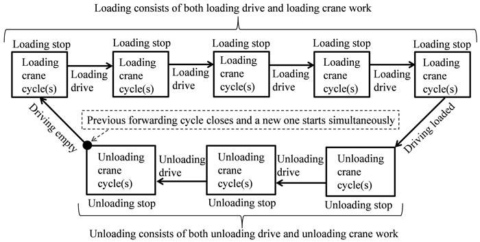
Fig. 1. Work element determination in the TimberLink system.
An ongoing Loading- or Unloading crane cycle ends and a new one starts simultaneously when the grapple is removed from the load-space after the grapple is opened. Possible sorting work in the load-space is included in the ongoing crane cycle. Moreover, crane work pauses longer than two seconds close an ongoing crane cycle, thus (for instance) returning the boom back to the load-space or simply dangling the grapple without moving the boom ends an ongoing crane cycle if the two-second threshold is passed.
As already mentioned PM time only includes effective working time (IUFRO 1995), as illustrated in Fig. 2. TimberLink extracts crane work PM time directly from the CAN-bus, rather than applying HMMs as for most variables. However, not all crane work is recognized as a crane cycle (either loading or unloading), but even in such cases it is all included in crane work time (Fig. 2). Moreover, some sporadic Loading crane cycles may be occasionally recognized during Unloading, and conversely some Unloading crane cycles may be recognized during Loading. These unexpected crane cycles are not documented as crane cycles, but as Loading- or Unloading crane work PM time, depending on the ongoing work element (i.e. preceding and subsequent crane cycles, Fig. 1). Thus, the crane work PM time is expected to be slightly higher than the crane cycle PM time for both Loading and Unloading.
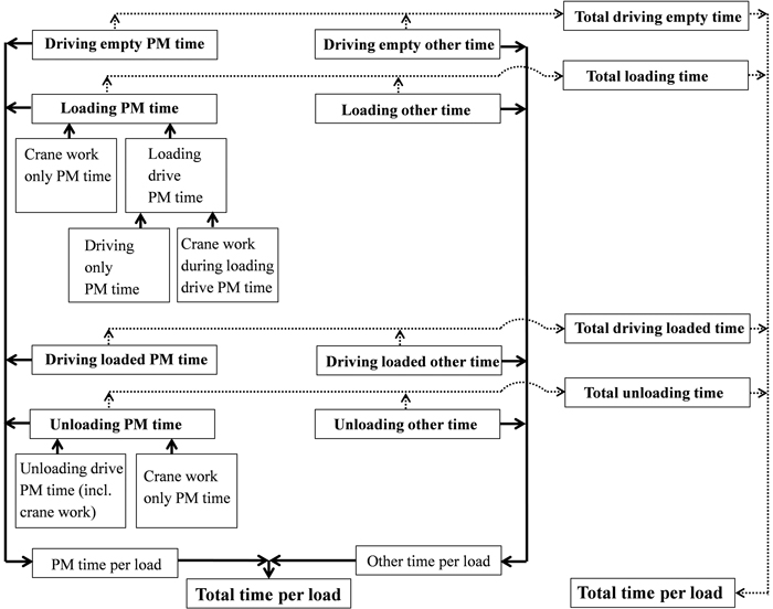
Fig. 2. Two ways to derive the total time per forwarded load; keeping PM (productive machine) time and other time separated (thicker contiguous flow line), or pooling PM and total time for each of four work elements (thinner flow line marked with dots).
Driving events between the first and last Loading crane cycles are defined as Loading drive, and similarly driving events between the first and last Unloading crane cycles are defined as Unloading drive. Driving between the last Unloading crane cycle and first Loading crane cycle is defined as Driving empty, and similarly driving between the last Loading crane cycle and first Unloading crane cycle is defined as Driving loaded. Generally, possible preparation time between a driving event and crane work, when neither driving nor crane work occur, is included in Other time.
Driving pauses (speed = 0) are excluded from all the speed observations and the speed is measured only when it is nonzero (speed > 0). Driving pauses are included in Total driving empty time and Total driving loaded time, but excluded from the respective PM times. Moreover, driving pauses are excluded from Loading drive and Unloading drive times, which are given as PM times.
Total time includes all time when the engine is running. Other time includes interruptions and micro-pauses provided that the engine is running. There is no minimum length for micro-pauses, but in practice the threshold is determined by the frequency of CAN-bus signals, thus even pauses lasting fractions of seconds will be registered as micro-pauses.
One full load (as a unit of observation) always includes at least six Loading- and six Unloading crane cycles. If this condition is not fulfilled, the load in question will be defined as an incomplete load, and all the associated observations will be merged with observations collected during the next load until it is fulfilled.
In summary, it should be noted that TimberLink generally recognizes work elements based on probabilistic methodology, i.e. choosing the most likely alternative.
2.3 Data analysis
All data were pooled over machines and operators to obtain general overall load-level results. Time consumption was analysed per load for Crane work only (with no simultaneous driving), Driving only (with no simultaneous crane work) and Simultaneous crane work and driving, as well as for the four work elements Driving empty, Loading, Driving loaded and Unloading. As driving and crane work can occur simultaneously, successive work elements may overlap (Fig 1). Speeds, distances, numbers and time consumptions of crane cycles, and proportions of Simultaneous crane work and driving per load were also analysed. However, TimberLink data do not provide specific indications of extraction distance (i.e. forwarding or forest transport distance), which was therefore defined as the mean of Driving empty and Driving loaded distances for each load.
From the data, means, standard deviations (SD), medians, median absolute deviations (MAD), and 5th, 25th, 75th and 95th percentiles of mentioned variables were calculated, with no removal of possible outliers. SD describes the dispersion of the dataset’s tails, i.e. how spread out the data tails are. While, MAD describes the data dispersion in general; the MAD’s difference from SD is that MAD does not give undue weight to the tail behaviour. Both SD and MAD were calculated according to the formulas presented in NIST/SEMATECH… (2013).
One-way analysis of variance (ANOVA) with Tukey’s simultaneous test of means was used to analyse the effect of driving phase (three levels: Driving empty, Loading drive and Driving loaded) on the driving speed, using general linear model (GLM) procedures in Minitab 17 (Minitab Ltd.). Differences in mean numbers of crane cycles during Loading and Unloading were tested using a paired sample t-test. In addition, relationships between the work elements’ time consumption (dependent variables) and extraction distance (independent variable) were explored by linear regression analysis. Spearman’s rank correlation coefficient (rs) was used to assess associations between driven distances and time consumption.
If data did not meet homoscedasticity and normality of distribution requirements for the ANOVA, paired sample t-test or linear regression analysis (according to ocular inspection of distributions and residual plots), they were transformed accordingly.
If logarithmically transformed data were used in the regression analyses, the constructed regression models were back-transformed after the analyses and multiplied by a correction factor to avoid logarithmic bias. The correction factor (q) was determined separately for each model as the ratio between sums of observed values, ![]() and predicted values,
and predicted values, ![]() (Eq. 1) (Holm 1977; Smith 1993).
(Eq. 1) (Holm 1977; Smith 1993).
The critical level of significance was set to 5%. Statistical analyses were performed using Minitab 17 (Minitab Ltd.) and RStudio version 3.0.1 (The R Foundation for Statistical Computing).
3 Results
In general variance in data varied from the level of 20% (SD) and 10% (MAD) for crane cycle times to the level of 450% (SD) and 90% (MAD) for Unloading other time (Tables 1 and 2). In addition, the data were positively skewed, except the speed and number of Unloading crane cycles observations, which were normally distributed (Tables 1 and 2). The data did not show a multimodal distribution despite data from several operators were pooled.
| Table 1. Forwarding time consumption (minutes/load). Total time consumption consists of productive machine (PM) time and other time. Means and medians are respectively followed by standard deviations (SD) and median absolute deviations (MAD) in brackets. In addition, 5th, 25th, 75th and 95th percentiles are given to provide general indications of the distribution of observations for each work element. The unit of observation is one load and unit of analysis is a minute per load. The number of observations varied from 8555 to 8868. | ||||||
| Percentiles | ||||||
| Work element | Mean, SD | Median, MAD | 5th | 25th | 75th | 95th |
| Total driving empty time | 7.0 (7.7) | 5.2 [3.2] | 0.3 | 2.5 | 9.1 | 19.1 |
| Driving empty PM time | 4.3 (3.6) | 3.5 [2.1] | 0.2 | 1.7 | 5.9 | 11.1 |
| Driving empty other time | 2.3 (5.8) | 0.5 [0.5] | 0.0 | 0.1 | 2.3 | 9.3 |
| Total loading time | 22.9 (16.0) | 19.9 [6.6] | 8.5 | 13.9 | 27.6 | 45.5 |
| Loading PM time | 21.0 (11.8) | 18.8 [6.1] | 8.2 | 13.4 | 25.9 | 40.0 |
| Loading other time | 1.9 (7.3) | 0.5 [0.4] | 0.1 | 0.2 | 1.4 | 7.7 |
| Crane work only PM time | 14.3 (7.2) | 13.0 [3.7] | 6.0 | 9.7 | 17.4 | 26.2 |
| Simultaneous crane work and driving a) | 1.4 (1.5) | 0.9 [0.6] | 0.1 | 0.4 | 1.9 | 4.2 |
| Driving only PM time b) | 5.3 (5.0) | 4.2 [2.2] | 0.7 | 2.3 | 6.8 | 13.2 |
| Loading drive PM time = a + b) | 6.7 (5.7) | 5.6 [2.7] | 1.1 | 3.1 | 8.7 | 16.0 |
| Total driving loaded time | 4.8 (4.2) | 3.7 [2.2] | 0.5 | 1.8 | 6.5 | 12.7 |
| Driving loaded PM time | 3.8 (3.6) | 2.8 [1.9] | 0.1 | 1.2 | 5.3 | 11.1 |
| Driving loaded other time | 0.6 (1.6) | 0.3 [0.2] | 0.0 | 0.1 | 0.6 | 2.0 |
| Total unloading time | 10.2 (9.9) | 8.2 [2.5] | 3.7 | 6.0 | 11.3 | 23.0 |
| Unloading PM time | 8.8 (5.8) | 7.5 [2.2] | 3.5 | 5.6 | 10.2 | 18.8 |
| Unloading other time | 1.4 (6.2) | 0.3 [0.3] | 0.0 | 0.1 | 1.1 | 4.7 |
| Crane work only PM time | 7.4 (3.8) | 6.8 [1.7] | 3.2 | 5.2 | 8.8 | 13.4 |
| Unloading drive PM time 1) | 1.4 (2.8) | 0.5 [0.4] | 0.0 | 0.2 | 1.5 | 6.1 |
| Total time per load | 45.8 (24.1) | 42.1 [11.8] | 19.1 | 31.0 | 55.3 | 84.5 |
| PM time | 39.3 (17.4) | 36.8 [10.1] | 17.3 | 27.5 | 48.2 | 68.2 |
| Other time | 6.5 (11.9) | 3.4 [2.2] | 0.6 | 1.6 | 7.1 | 21.6 |
| 1) Can also include simultaneous crane work | ||||||
| Table 2. Descriptive forwarder work variables. Means and medians are respectively followed by standard deviations (SD) and median absolute deviations (MAD) in brackets. In addition, 5th, 25th, 75th and 95th percentiles are given. The unit of observation is one load. | |||||||
| Percentiles | |||||||
| Variable | Sort | Mean, SD | Median, MAD | 5th | 25th | 75th | 95th |
| Driving empty distance | m/load | 256.3 (234.5) | 199.4 [129.3] | 4.9 | 90.6 | 358.1 | 702.1 |
| Loading drive distance | m/load | 236.8 (255.3) | 183.0 [91.0] | 37.3 | 102.5 | 289.3 | 596.1 |
| Driving loaded distance | m/load | 181.3 (171.8) | 134.8 [95.7] | 3.1 | 52.4 | 262.4 | 524.2 |
| Unloading drive distance | m/load | 71.4 (166.4) | 18.6 [17.2] | 0.0 | 4.3 | 72.4 | 305.4 |
| Extraction distance 1) | m/load | 219.0 (177.5) | 173.9 [99.8] | 24.8 | 87.6 | 302.1 | 578.6 |
| Total driven distance | m/load | 779.8 (518.5) | 666.2 [275.0] | 197.2 | 425.5 | 1006.8 | 1720.2 |
| Driving empty speed 2) | km/h | 3.4a (1.0) | 3.3 [0.5] | 1.8 | 2.8 | 3.9 | 5.1 |
| Loading drive speed | km/h | 2.1b (0.5) | 2.0 [0.3] | 1.3 | 1.7 | 2.4 | 3.0 |
| Driving loaded speed | km/h | 2.9c (0.8) | 2.8 [0.5] | 1.6 | 2.4 | 3.4 | 4.4 |
| Loading crane cycle numbers 3) | cycles/load | 34.9a (12.0) | 34.0 [7.0] | 17.0 | 27.0 | 42.0 | 56.0 |
| Unloading crane cycle numbers | cycles/load | 16.7b (5.9) | 16.0 [3.0] | 9.0 | 13.0 | 20.0 | 25.0 |
| Loading crane cycle time | s/cycle | 23.7 (5.2) | 22.5 [2.8] | 17.6 | 20.2 | 26.2 | 33.3 |
| Unloading crane cycle time | s/cycle | 23.4 (5.3) | 22.5 [3.0] | 16.9 | 19.8 | 25.9 | 33.0 |
| Proportion of crane work during loading drive PM time | % | 22.1 (16.3) | 18.3 [9.1] | 3.1 | 10.4 | 29.8 | 53.8 |
| 1) Extraction distance = mean of Driving loaded and Driving empty distances. 2) Different superscript letters within speed variables indicate significant differences (p < 0.001, one-way ANOVA with Tukey test, n = 8868). 3) Different superscript letters within crane cycle numbers indicate significant differences (p < 0.001, paired t-test, n = 8868). Differences between the pairs were normally distributed. | |||||||
Every work element’s time consumption (PM and total) per load was dependent on the extraction distance (Table 3, p < 0.001, Fig. 3). The constructed models explained large proportions of the total variation of Driving empty PM time and Driving loaded PM time (Table 3, 52.8% < R-Sq(adj.) < 61.8%), but minor proportions of the total variation of Loading and Unloading time consumptions (Table 3, 1.5% < R-Sq(adj.) < 2.6%). Moreover, Other time in total was weakly dependent on extraction distance (Table 3, R-Sq(adj.) = 4.8%, Fig. 5). The mean and median total driven distances were 780 and 666 m, respectively (Table 2). Corresponding extraction distances were 219 and 174 m (Table 2), and in the range between those values Loading, Unloading, Driving empty and Driving loaded PM time accounted for on average ca. 46, 19, 9 and 8% of total forwarding time consumption, respectively, while Other time accounted for ca. 14% (Figs. 3 and 4). The average and median total time consumptions were 45.8 and 42.1 minutes per load.
| Table 3. Forwarding time consumption (second/load) in total (Tot.), during PM work and during Other time (Other) as functions of extraction distance (Ext.Dist.) (metre). Models were also derived separately for work elements Driving empty (D.E.), Loading (L.), Driving loaded (D.L.) and Unloading (Unl.). SE = standard error, n = number of loads, S = standard error of the estimate. Ext.Dist. = mean of Driving loaded and Driving empty distances. | |||||||||
| Dependent variable | Predictor | Coefficient | SE coeff. | T-value | Model | Bias correction | |||
| F | R2(adj) (%) | S | n | ||||||
| Ln(Tot.) | Ln(Ext.Dist.) | 0.20568 | 0.00440 | 46.70 | 2180.63 | 19.8 | 0.412911 | 8857 | 1.09104 |
| Constant | 6.7821 | 0.0225 | 301.25 | ||||||
| Ln(PM) | Ln(Ext.Dist.). | 0.20492 | 0.00403 | 50.85 | 2585.46 | 22.6 | 0.377802 | 8857 | 1.07189 |
| Constant | 6.6508 | 0.0206 | 322.87 | ||||||
| Ln(Tot. Other) | Ln(Ext.Dist.) | 0.2438 | 0.0116 | 21.06 | 443.57 | 4.8 | 1.08514 | 8856 | 1.85197 |
| Constant | 4.1012 | 0.0592 | 69.32 | ||||||
| Ln(D.E. Tot.) | Ln(Ext.Dist.) | 0.82937 | 0.00895 | 92.71 | 8594.49 | 49.3 | 0.837579 | 8843 | 1.27755 |
| Constant | 1.3692 | 0.0457 | 29.93 | ||||||
| Ln(D.E. PM) | Ln(Ext.Dist.) | 0.91374 | 0.00772 | 118.36 | 14009.34 | 61.8 | 0.692162 | 8676 | 1.13247 |
| Constant | 0.5266 | 0.0396 | 13.28 | ||||||
| Ln(L. Tot.) | Ln(Ext.Dist.) | 0.07133 | 0.00575 | 12.41 | 153.91 | 1.7 | 0.539013 | 8857 | 1.16125 |
| Constant | 6.7165 | 0.0294 | 228.54 | ||||||
| Ln(L. PM) | Ln(Ext.Dist.) | 0.08332 | 0.00539 | 15.45 | 238.80 | 2.6 | 0.505486 | 8857 | 1.13196 |
| Constant | 6.5926 | 0.0276 | 239.20 | ||||||
| Ln(D.L. Tot.) | Ln(Ext.Dist.) | 0.67811 | 0.00797 | 85.06 | 7235.81 | 45.0 | 0.747323 | 8857 | 1.24241 |
| Constant | 1.8581 | 0.0407 | 45.60 | ||||||
| Ln(D.L. PM) | Ln(Ext.Dist.) | 0.85758 | 0.00877 | 97.73 | 9551.91 | 52.8 | 0.770664 | 8555 | 1.23240 |
| Constant | 0.6436 | 0.0452 | 14.25 | ||||||
| Ln(Unl. Tot.) | Ln(Ext.Dist.) | 0.06774 | 0.00589 | 11.50 | 132.34 | 1.5 | 0.552018 | 8857 | 1.19892 |
| Constant | 5.8954 | 0.0301 | 195.87 | ||||||
| Ln(Unl. PM) | Ln(Ext.Dist.) | 0.07086 | 0.00526 | 13.48 | 181.77 | 2.0 | 0.492719 | 8857 | 1.14050 |
| Constant | 5.7843 | 0.0269 | 215.31 | ||||||
| Ln(D.E. Other) | Ln(Ext.Dist.) | 0.7479 | 0.0228 | 32.77 | 1073.97 | 11.3 | 2.02959 | 8402 | 4.12739 |
| Constant | –0.420 | 0.118 | –3.58 | ||||||
| Ln(L. Other) 1) | Ln(Ext.Dist.) | –0.0165 | 0.0158 | –1.05 | 1.09 | 0.0 | 1.47879 | 8853 | 3.38023 |
| Constant | 3.6225 | 0.0807 | 44.91 | ||||||
| Ln(D.L. Other) | Ln(Ext.Dist.) | 0.2328 | 0.0174 | 13.40 | 179.43 | 2.1 | 1.57333 | 8508 | 2.74649 |
| Constant | 1.3921 | 0.0892 | 15.60 | ||||||
| Ln(Unl. Other) | Ln(Ext.Dist.) | 0.0677 | 0.0183 | 3.70 | 13.66 | 0.1 | 1.71746 | 8854 | 4.51765 |
| Constant | 2.5647 | 0.0937 | 27.38 | ||||||
| p-value < 0.001 for all the coefficient estimates (including both ln(Ext.Dist) and constant) and models – 1)except, p = 0.296 for both Ln(Ext.Dist) and the model. When estimating dependent variables, the predicted dependent variable may be multiplied by the given correction factor for logarithmic bias (i.e. bias correction). For example: Driving empty = 1.27755×exp(1.3692 + 0.82937×ln(Ext.Dist.)). | |||||||||
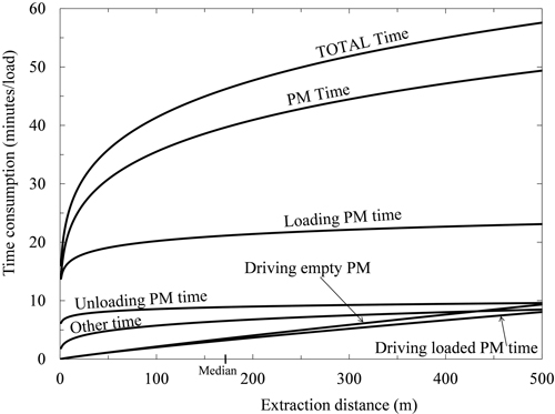
Fig. 3. The total and productive machine time (PM time) consumption as a function of extraction distance (mean of Driving unloaded and Driving loaded distances). The median extraction distance is marked on the horizontal axis (see Table 2). PM time is also shown for each of the four work elements Loading (crane work and driving included), Unloading (crane work and driving included), Driving empty, Driving loaded, and Other time. Applied models are taken from Table 3 and corrected for logarithmic bias.
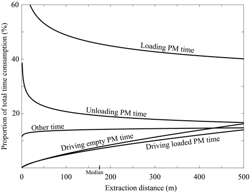
Fig. 4. PM times’ proportions of total time consumption as a function of extraction distance (mean of Driving loaded and Driving unloaded distances). The median extraction distance is marked on the horizontal axis (see Table 2). Applied models are taken from Table 3 and corrected for logarithmic bias.
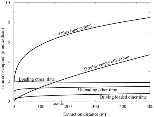
Fig. 5. Other time as a function of extraction distance (mean of Driving loaded and Driving unloaded distances). The median extraction distance is marked on the horizontal axis (see Table 2). Total other time is also shown for each of the four work elements Loading (crane work and driving included), Unloading (crane work and driving included), Driving empty and Driving loaded. Applied models are taken from Table 3 and corrected for logarithmic bias.
Based on mean values, the crane was used during 74.8% of Loading PM time, the driving speed was nonzero during 31.9% of Loading PM time, Simultaneous crane work and driving occurred during 6.7% of Loading PM time (Table 1) and the crane was used during 22.1% of Loading drive PM time (Table 2). Also based on means (Table 2), Driving empty and Driving loaded accounted for 56.2% of the total driven distance, while Loading drive and Unloading drive accounted for 39.5% of the total driven distance and 4.3% could not be classified. In addition, cumulative distance distribution curves were positively skewed for all the studied distances (cf. Table 2 and Fig. 6). The skew was most pronounced for the Unloading drive distance and mildest for total driven distance.
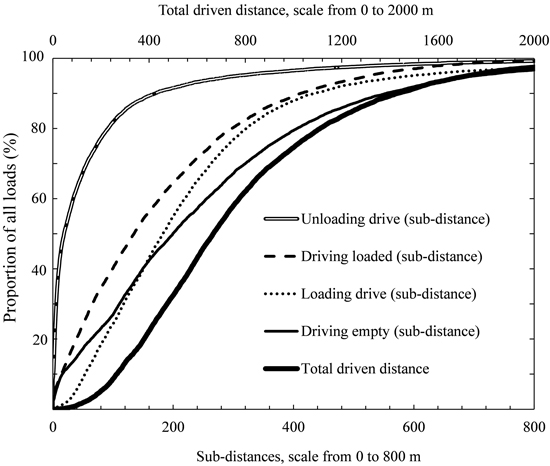
Fig. 6. Cumulative distribution of distances driven during indicated work elements required to fulfil a load (including all work elements pooled, i.e. total driven distance). For instance, ca. 90% of all loads had an Unloading drive distance less than 200 m per load and ca 40% of all loads had a total driving distance less than 600 m per load.
For 96% of all studied loads Driving empty and Driving loaded PM time accounted for less than 22 and less than 25% of total time consumption, respectively (Fig. 7). For 10% of all studied loads Loading PM time accounted for less than 30% of total time consumption, while for slightly over 80% of the loads it accounted for 30–65% of total time consumption. For 90% of the studied loads Unloading PM time accounted for less than 32% of total time consumption. Other time also accounted for less than 25% of total time consumption for 90% of the studied loads (Fig. 7).
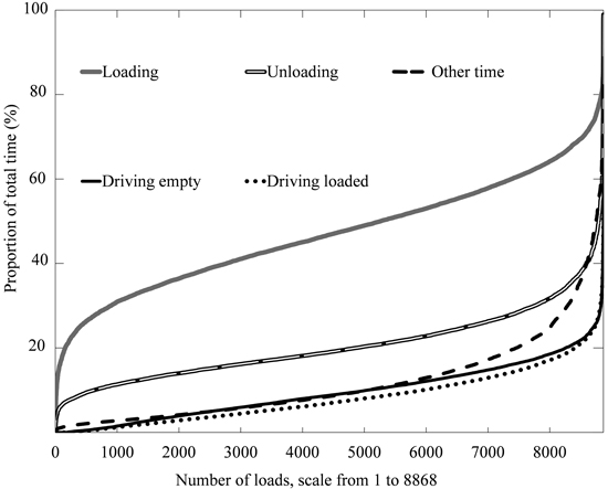
Fig. 7. Work elements’ relative proportions of total time consumption during forwarding of a load, ordered according to size of proportion size within each work element. The total number of observations (loads) is 8868. For instance, for approximately half of the loads, the Loading PM time constituted 40–60% of the total time (for ca. 7000 observations the proportion was equal to or less than 60%, and for ca. 3000 observations it was equal to or less than 40%; 7000–3000 = 4000). Similarly, for more than 8000 of the observations, the relative time spent on Driving empty was below 20% of the total time spent on forwarding the load.
Driving empty speed was on average fastest among the driving speeds (Table 2). The average Driving empty speed (3.4 km/h) was 17% faster than the average Driving loaded speed, and 62% faster than the average Loading drive speed (One-way ANOVA, p < 0.001, n = 8868).
Loading and Unloading crane cycle times were nearly identical, on average 23.4–23.7 seconds (Table 2). However, on average Loading included approximately twice as many crane cycles (34.9) as Unloading (16.7), hence the average handled timber volume was approximately twice as large during an Unloading crane cycle than during a Loading crane cycle (Table 2, paired t-test, p < 0.001, n = 8868).
Loading drive distance correlated positively with both total time per load (rs = 0.539) and PM time per load (rs = 0.572), as did extraction distance, but slightly less strongly (rs = 0.473 and 0.495, respectively). Thus, time consumption per load was more closely associated with Loading drive distance than with extraction distance.
4 Discussion
This study contributes both knowledge on possibilities that the new data gathering technology provides, and representative data on forwarding time consumption of unprecedented quantity and resolution. Such information is crucial for applications such as robust simulations, costing and developing forwarding decision support systems. In a literature review by Manner et al. (2013) it was found that if forwarding cycles are divided into four work elements, with an extraction distance of 200 m (single-way), Loading, Unloading, Driving empty and Driving loaded (pooled) and Loading drive account for ca. 45, 25, 15 and 10% of total time consumption, respectively. Our results corroborate these findings, as Driving empty and Driving loaded collectively consumed only 15–20% of the total forwarding time, while Loading and Unloading collectively consumed 80–85% of the total time.
Previously recorded speed observations vary considerably, but those reported here for the specified driving phases are consistent with recent literature, which display no chronological trend of increasing or decreasing speed (cf. Väkevä et al. 2001; Nurminen et al. 2006; Table 2).
Previously reported Driving empty and Loaded distances also vary considerably, but on average our distance observations are consistent with current literature (cf. Kellogg and Bettinger 1994; McNeel and Rutherford 1994; Nurminen et al. 2006; Table 2). However, the average Loading drive distance we observed was twice or triple as long as corresponding distances reported by Nurminen et al. (2006) and Kellogg and Bettinger (1994). The short Loading drive distance reported by Kellogg and Bettinger (1994) can be partly explained by high forwarded log concentrations, while the long Loading drive distances in our study can be partly explained by the fact that the studied forwarders had a larger load capacity than those used in the cited studies.
In our study the PM time consumption per load increased by roughly 10% per 100 m increase in extraction distance for distances over 100 m, in accordance with previous studies (cf. e.g. Kellogg and Bettinger 1994). Tiernan et al. (2004) found that the PM time increased even more, by ca. 15% per 100 m increase in extraction distance, but they defined the extraction distance as half of the total driven distance. Hence, their definition included distances of Loading and Unloading drive, during which speed is lower (Table 2) and consequently the work takes longer.
Extraction distance is the most important factor in current productivity norms and studies (see e.g. Kahala and Kuitto 1986; Kuitto 1990, 1992; MoDo Skog 1993; Brunberg 2004; Hakonen 2013). However, we found that forwarding time consumption is relatively weakly correlated with extraction distance, and more closely associated with Loading drive distance. The Loading drive distance depends on forwarded log concentration, which in turn depends on assortment volumes and distributions at the harvesting site, and the assortments loaded in one load (Manner et al. 2013). Thus, for productivity estimates, assortment volumes and distributions at the harvesting site should be taken into account more rigorously, which is already possible using spatial harvester data (see, e.g., Nordström et al. 2006; Arlinger et al. 2012; Möller et al. 2013). The relevance of extraction distance as the main indicator for forwarding productivity should also be critically discussed, especially as the concept ‘extraction distance’ is ambiguously defined and difficult to assess adequately in practice (see Eriksson and Lindroos 2014; Manner 2015).
As forest work conditions vary substantially, important variables such as log concentration, ground-bearing capacity, numbers of assortments, weather and time of year should also ideally be taken into account when analysing forwarding work (see, e.g., Asserståhl 1973; Väkevä et al. 2001; Kuitto 1990, 1992; Kuitto et al. 1994; Nurminen et al. 2006; Manner et al. 2013; Eriksson and Lindroos 2014). In our study we lacked information on many of those variables, which is a limitation for our regression analyses (Figs. 3–5, Table 3), as they presumably influenced the observed time consumptions in uncontrolled ways. However, intuitive expectations and cited literature suggest that time consumptions and extraction distances are associated. Moreover, the dataset used was large (covering 8868 loads forwarded by nine operators), included observations for only one forwarder model, and covered all typical final felling work conditions in every time of year in mid Sweden. Therefore, the possible effects of nuisance factors on the representativeness of the regression models were probably minor.
In productivity-oriented follow-up studies measurements are typically expressed per unit volume (see, e.g., Eriksson and Lindroos 2014). However, if the objective is to elucidate elements of work cycles measurements per load, such as those presented here, are better. For instance, information on driving distances and time consumptions per unit volume provide much less clear understanding of work elements than information on the same variables per load.
A strength of this study is that the data are work element-specific and unusually representative for real life work. Both forwarders were of the same brand and model, of the largest size-class of forwarders on the market. All data pertain to operations in final fellings in a specific region with terrain conditions varying from easy to moderate, and all nine operators were experienced. Furthermore, data were collected for more than two years, thus operations in all kinds of weather in both summer and winter conditions are represented in the data. Since sample-sizes were large, trends and distributions can be considered as representative for final felling operations in the study area.
Another strength of the study is the inclusion of overlapping work elements. In a conventional time study the forwarding work elements’ definitions are based solely on visual cues (e.g. tyre rotation) and they are roughly divided for practical convenience. Thus, for instance, short pauses between work elements are not recognized and work elements cannot overlap (see, e.g., Väkevä et al. 2001; Tiernan 2004; Manner et al. 2013). However, Väkevä et al. (2001) recorded PM and PM15 times (which include PM times and up to 15-minute interruptions) separately. Several previous authors, e.g. Kuitto et al. (1994), Kellogg and Bettinger (1994) and Nurminen et al. (2006), have based work element definition on both tyre rotation and crane usage, as in our study. In such cases, the observer must deal with possibly overlapping work elements and Other time (i.e. time when neither drive nor crane use occur). Kuitto et al. (1994) addressed the latter problem in a similar fashion to us, by determining Other time as a separate work element, and found that it accounted for 6.5% of PM15 time when the ground was snow-free and 8.6% when the ground was covered by snow. Väkevä et al. (2001) found that interruptions accounted for 10.8% of PM15 time in final felling operations and 11.5% in thinning operations, including observations in both snow-free and snow-covered ground conditions. The interruptions and Other time reported by Kuitto et al. (1994) and Väkevä et al. (2001) are somewhat shorter than our findings, but this is consistent with expectations because we extracted Other time from CAN-bus data, which catch Other time elements such as pauses (and other work elements) that last even fractions of seconds, while the manual timing methods applied by Kuitto et al. (1994) and Väkevä et al. (2001) inevitably have much lower resolution. Hence, some of what is defined as Other time in our study would be missed (or rather allocated to other work elements) with lower resolution manual data gathering.
A weakness of the study is the lack of information on specific stand conditions (terrain conditions, volume per ha, number of assortments) and load sizes during the recordings, and how the operators planned their work. However, the stem-volume is on average 200–210 m3 per ha in stands aged 80 to 140 years (the usual final felling age range) in this part of Sweden (see Kempe 2014). According to a classification by von Segebaden (1975) the average surface roughness of forest land in this region varies from 1.2 to 2.9 (where 1 is “very smooth” and 5 is “very uneven”), while inclination varies from 1.0 to 1.6 (where 1 refers to inclinations less than 10%, and 5 to inclinations more than 51%) and ground-bearing conditions vary from 1.9 to 3.0 (where 1 is “very good” and 5 is “very poor”; cf. Berg 1982). Thus, generally the terrain conditions were relatively good.
A typical load-size for the studied forwarder can be estimated, in m3, as follows. Logs (both pulpwood and sawlogs) are ca. 4.6 m long in this region, and the load density is 55–60% (Magnus Haapaniemi, Quality and control VMF Qbera, Falun, pers. comm. in 2015). As the load-area was 6.2 m2 a full load varied roughly from 15.8 to 17.2 m3 in solid volume. Assuming that the average load was in the range of 90–100% of these volumes, the average productivity was in the range of 20–24 m3 solid volume/hour when the engine was running (see Table 3). This productivity estimate is consistent with contemporary data on forwarding in final felling operations (see Eriksson and Lindroos 2014).
To conclude, this study is representative for work with large forwarders in final felling operations in areas with typical terrain conditions for mid-Sweden (see von Segebaden 1975; Berg 1982), although stand-specific characteristics were not available for the collected dataset.
Forwarders’ on-board computers (also TimberLink) define distance, and thereby also speed, based on the angular velocity of drive axles. Thus, depending on terrain conditions, presented driving distances and speeds might be slight overestimations due to wheel slip. Use of GNSS application has been suggested to deal with distance overestimation caused by the wheel slip (see e.g. Suvinen et al. 2006). This could be a sound option on even ground but not in forest where the machine has to run over small obstacles; use of GNSS application would lead to notable distance underestimations as it misses the extra distance that machine has to travel to run over obstacles (Ringdahl et al. 2012). However, possible distance overestimation does not have any direct influence on presented time consumption figures (Tables 1 and 2). Instead, extraction distances in Figs. 3–5 and in Table 3 might be overestimations. But the effect of possible overestimation is linear, meaning that its relative effect on time consumption predictions is constant over the studied distance range. Moreover, the effect of possible overestimation is equal between the work elements (Figs. 3–5, Table 3).
Probabilistic work element recognition based on use of Viterbi algorithms is reportedly robust when the observed work is clearly cyclic (Palmroth 2011). Forwarding of single-assortment loads can be considered cyclic in this context, with minor exceptions such as occasional accumulation of piles within the loading crane cycle. However, other parts of the work are clearly non-cyclic, for instance the abundant assortment sorting when unloading multi-assortment loads, which involves both unloading and loading crane cycles, and diverse kinds of crane work. Thus, the dataset used in this study may include some erroneous classifications due to errors in work element and load recognitions, but the data were not filtered since it was not known if outliers were measurement errors or extreme observations and possibly essential parts of forwarder work. Nevertheless, the applied log transformation effectively normalized the data distributions and harmonized the variance. Thus, the outliers’ effects on the ANOVA results were minor or non-existent.
Log transformation creates curvilinear relationships, which makes interpretation of graphical results more complicated (e.g. Osborne 2002). Thus, it is doubtful whether curvilinear relationships between dependent and independent variables shown in Fig. 3 are accurate, and both linear and curvilinear relationships have been presented in previous studies (see, e.g., Kuitto et al. 1994; Kellogg and Bettinger 1994; Väkevä et al. 2001; Nordfjell et al. 2003; Brunberg 2004; Tiernan et al. 2004; Nurminen et al. 2006; Manner et al. 2013). Erroneous curvilinearity would lead to errors in estimations, depending on the extraction distance (cf. Table 1; Fig. 3). However, we found relations between time consumptions for individual work elements and extraction distances to be close to linear, for extraction distances over 100 m, even with the curvilinear model we used (Fig. 3).
4.1 Conclusions
Using time consumption data derived from forwarders’ CAN-bus messages was found to be an informative option for research purposes. They can provide records of elements lasting just fractions of a second, and in the same databases information spanning long time periods covering operations with many machines. This enables time consumption readings, for example, for single crane cycles at load level during a whole year of work. It should be noted that although forwarder CAN-bus data provide access to variables such as steering, speed and crane use, the raw data do not directly show what the machine was being used for at a given time, for instance Loading or Unloading. TimberLink data were found to be intuitively logical and to give results in line with current literature. However, further study is warranted to confirm TimberLink’s capability to determine work elements correctly, especially for multi-assortment loads.
Total and PM time consumptions were clearly correlated with Loading drive distances. However, elucidating effects and interactions of predictive variables and operator behaviour on time consumptions is not straightforward, and requires datasets with more detailed information about loads (e.g. volumes and numbers of assortments) and stand conditions (e.g. volumes per ha and per unit strip road distance, as well as terrain conditions).
Acknowledgements
This study was funded by Stora Enso Skog AB and the Forest Industrial Research School on Technology (FIRST).
References
Andersson A. (2015). En analysmodell för tidsåtgång vid skotning med Komatsuskotare. [An analysis model for time consumption while forwarding with Komatsu forwarders]. Master’s thesis. The Swedish University of Agricultural Sciences, Department of Forest Biomaterials and Technology. 42 p. [In Swedish, English summary].
Arlinger J., Möller J., Sorsa J.-A., Räsänen T. (2012). Introduction to StanForD2010. Structural descriptions and implementation recommendations. Skogforsk. 74 p. [Published draft].
Asserståhl R. (1973). Terrängtransport med skotare. [Off-road transport by forwarders: analysis of effects of various terrain factors on travel speed]. Skogforsk, Redogörelse 2. 20 p. [In Swedish].
Berg S. (1982). Terrängtypsshema för skogsarbete. [Terrain classification scheme for forestry work]. Skogforsk. 28 p. [In Swedish].
Bergstrand K.-J. (1985). Underlag för prestationsmål för skotning. [Productivity norm for forwarding]. Skogforsk, Redogörelse 7. 27 p. [In Swedish].
Brunberg T. (2004). Underlag till produktionsnormer för skotare. [Productivity-norm data for forwarders]. Skogforsk, Redogörelse 3. 12 p. [In Swedish, English summary].
Cordero R., Mardones O., Marticorena M. (2006). Evaluation of forestry machinery performance in harvesting operations using GPS technology. In: Ackerman P.A., Längin D.W., Antonides M.C. (eds.). Precision forestry in plantations, semi-natural and natural forests. Proceedings of the International Precision Forestry Symposium, Stellenbosch, Stellenbosch University.
Eriksson M., Lindroos O. (2014). Productivity of harvesters and forwarders in CTL operations in Northern Sweden based on large follow-up datasets. International Journal of Forest Engineering 25: 179–200. http://dx.doi.org/10.1080/14942119.2014.974309.
Gerasimov Y., Senkin V., Väätäinen K. (2012). Productivity of single-grip harvesters in clear-cutting operations in the northern European part of Russia. European Journal of Forest Research 131: 647–654. http://dx.doi.org/10.1007/s10342-011-0538-9.
Gullberg T. (1995). Jämförande experimentella studier av lantbrukstraktor med griplastarvagn och liten skotare. [Comparative experimental studies of farm tractors with grapple-loader trailers and a small forwarder]. Doctoral thesis. Swedish University of Agricultural Sciences, Department of Operational Efficiency. 71 p. [In Swedish, English summary].
Hakonen O. (2013). Metsäkuljetusmatkan arvioinnin erot puunostajan ja puunkorjuuyrittäjän välillä Stora Enso Metsän Itä-Suomen hankinta-alueella. [Differences assessing forest extraction distances between procurement supervisors and timber harvesting entrepreneurs in Stora Enso Eastern Finland Wood Supply]. Bachelor’s thesis. Karelia University of Applied Sciences. 41 p. [In Finnish, English summary].
Holm S. (1977). Transformationer av en eller flera beroende variabler i regressionsanalys. [Transformations of one or several dependent variables in regression analysis]. Swedish University of Agricultural Sciences, Faculty of Forest Sciences, HUGIN report No. 7. 21 p. [In Swedish].
Holzleitner F., Stampfer K., Visser R. (2011). Utilization rates and cost factors in timber harvesting based on long-term machine data. Croatian Journal of Forest Engineering 32: 501–508.
IUFRO WP 3.04.02 (1995). Forest work study nomenclature. Test edition valid 1995–2000. Department of Operational Efficiency, Swedish University of Agricultural Sciences. 16 p.
John Deere Forestry Oy (2008). In the forest. John Deere Forestry Oy’s customer magazine, Issue 2. 24 p. http://jd.smartpage.fi/itf208/pdf/ITF_2_08.pdf. [Cited 21 April 2015, In Finnish].
Kahala M., Kuitto P.-J. (1986). Puutavaran metsäkuljetus keskikokoisella kuormatraktorilla. [Forest haulage of timber using medium-sized forwarder]. Metsäteho, Katsaus. 4 p.
Kellogg L.D., Bettinger P. (1994). Thinning productivity and cost for mechanized cut-to-length system in the Northwest Pacific coast region of the USA. Journal of Forest Engineering 5: 43–52. http://dx.doi.org/10.1080/08435243.1994.10702659.
Kempe G. (2014). Forest and forest-land. In: Christiansen L. (ed.). Swedish statistical yearbook of forestry 2014. Swedish Forest Agency. p 41–70.
Kuitto P.-J. (1990). Metsäkuljetus harvesterin jälkeen. [Forest haulage after mechanized cutting]. Metsäteho, Katsaus. 6 p. [In Finnish, English summary].
Kuitto P.-J. (1992). Koneellinen hakkuu ja metsäkuljetus – maksuperusteselvitys 1990–1992. [Mechanized cutting and forest haulage]. Metsäteho, Katsaus. 8 p. [In Finnish, English summary].
Kuitto P.-J., Keskinen S., Lindroos J., Oijala T., Rajamäki J., Räsänen T., Terävä J. (1994). Puutavaran koneellinen hakkuu ja metsäkuljetus. [Mechanized cutting and forest haulage]. Metsäteho, Tiedotus 410. 38 p. [In Finnish, English summary].
Manner J. (2015). Automatic and experimental methods to studying forwarding work. Doctoral thesis. Swedish University of Agricultural Sciences, Acta Universitatis agriculturae Sueciae. ISBN 978-91-576-8454-7. 71 p. http://urn.kb.se/resolve?urn=urn:nbn:se:slu:epsilon-e-3069.
Manner J., Nordfjell T., Lindroos O. (2013). Effects of the number of assortments and log concentration on time consumption for forwarding. Silva Fennica 47(4) article 1030. http://dx.doi.org/10.14214/sf.1030.
Mayo E. (1933). The human problems of an industrial civilization. Macmillan Company, New York. 194 p.
McNeel J.F., Rutherford D. (1994). Modeling harvester-forwarder system performance in a selection harvest. Journal of Forest Engineering 6: 7–14. http://dx.doi.org/10.1080/08435243.1994.10702661.
Mederski P.S. (2006). A comparison of harvesting productivity and costs in thinning operations with and without midfield. Forest Ecology and Management 224: 286–296. http://dx.doi.org/10.1016/j.foreco.2005.12.042.
MoDo Skog (1993). Underlag för prestationsprognos, bortsättning. Skotare. [Productivity norm for forwarder]. 2 p. [In Swedish].
Möller J.J, Arlinger J., Nordström M. (2013). Test av StanForD 2010 – implementation i skördare. [StanForD 2010 – implementation and test of harvester]. Skogforsk, Arbetsrapport nr. 798. ISSN 1404-305X. 58 p. [In Swedish, English summary].
NIST/SEMATECH e-Handbook of Statistical Methods (2013). Section 1.3.5.6. Measures of scale. http://www.itl.nist.gov/div898/handbook/eda/section3/eda356.htm. [Cited 7 March 2016].
Nordfjell T., Athanassiadis D., Talbot B. (2003). Fuel consumption in forwarders. International Journal of Forest Engineering 14: 11–20.
Nordström M., Möller J., Larsson W., Arlinger J. (2006). Skördardata ger värdefull information om skogen. [Harvester data provides valuable information on the forest]. Skogforsk, Resultat nr. 10 2009. 4 p. [In Swedish, English summary].
Nurminen T., Korpunen H., Uusitalo J. (2006). Time consumption analysis of the mechanized cut-to-length harvesting system. Silva Fennica 40(2): 335–363. http://dx.doi.org/10.14214/sf.346.
Nuutinen Y. (2013). Possibilities to use automatic and manual timing in time studies on harvester operations. Doctoral thesis. University of Eastern Finland, School of Forest Sciences, Dissertationes Forestales 156. 68 p. http://dx.doi.org/10.14214/df.156.
Nuutinen Y., Väätäinen K., Heinonen J., Asikainen A., Röser D. (2008). The accuracy of manually recorded time study data for harvester operation shown via simulator screen. Silva Fennica 42(1): 63–72. http://dx.doi.org/10.14214/sf.264.
Osborne J. (2002). Notes on the use of data transformations. Practical Assessment, Research & Evaluation 8(6). 11 p. ISSN 1531-7714.
Palander T., Nuutinen Y., Kariniemi A., Väätäinen K. (2013). Automatic time study method for recording work phase times of timber harvesting. Forest Science 59(4): 472–483. http://dx.doi.org/10.5849/forsci.12-009.
Palmroth L. (2011). Performance monitoring and operator assistance systems in mobile machines. Doctoral thesis. Tampere University of Technology. Publication 955. ISBN: 978-952-15-2533-9. 110 p.
Purfürst F.T. (2010). Learning curves of harvester operations. Croatian Journal of Forest Engineering 31: 89–97.
Purfürst F.T., Erler J. (2011). The human influence on productivity in harvester operations. International Journal of Forest Engineering 22: 15–22.
Purfürst F.T., Lindroos O. (2011). The correlation between long-term productivity and short-term performance ratings of harvester operators. Croatian Journal of Forest Engineering 32: 509–519.
Sirén M. (1998). Hakkuukonetyö, sen korjuujälki ja puustovaurioiden ennustaminen. [One-grip harvester operation, its silvicultural result and possibilities to predict tree damage]. Doctoral thesis. The Finnish Forest Research Institute, Research Papers 694. ISBN 951-40-1635-1. 179 p. [In Finnish, English summary].
Skogforsk (2012). StanForD. Listing of variables by category. 141 p. http://www.skogforsk.se/contentassets/46bd88507c8343318d34523a7dfd6f4e/allvargrp_eng_120418.pdf. [Cited 16 September 2013].
Ringdahl O., Hellström T., Wästerlund I., Lindroos O. (2012). Estimating wheel slip for a forest machine using RTK-DGPS. Journal of Terramechanics 49(5): 271–279. http://dx.doi.org/10.1016/j.jterra.2012.08.003.
Smith R.J. (1993). Logarithmic transformation bias in allometry. American Journal of Physical Anthropology. p. 215–228.
Spinelli R., Magagnotti N., Pari L., De Francesco F. (2015). A comparison of tractor-trailer units and high-speed forwarders used in Alpine forestry. Scandinavian Journal of Forest Research 30(5): 470–477. http://dx.doi.org/10.1080/02827581.2015.1012113.
Strandgard M., Mitchell R. (2015). Automated time study of forwarders using GPS and a vibration sensor. Croatian Journal of Forest Engineering 36: 175–184.
Strandgard M., Walsh D., Acuna M. (2013). Estimating harvester productivity in Pinus radiata plantations using StanForD stem files. Scandinavian Journal of Forest Research 28(1): 73–80. http://dx.doi.org/10.1080/02827581.2012.706633.
Suvinen A. Saarilahti M. (2006). Measuring the mobility parameters of forwarders using GPS and CAN bus techniques. Journal of Terramechanics 43(2): 237–252. http://dx.doi.org/10.1016/j.jterra.2005.12.005.
Taylor S.E., McDonald T.P., Veal M.V., Grift T.E. (2011). Using GPS to evaluate the productivity and performance of forest machine systems. In: Briggs D. (ed.). Proceedings of the first international precision forestry co-operative symposium, Seattle, University of Washington. p. 151–156.
Tiernan D., Zeleke G., Owende P.M.O., Kanali C.L., Lyons J., Ward S.M. (2004). Effect of working conditions on forwarder productivity in cut-to-length timber harvesting on sensitive forest sites in Ireland. Biosystems Engineering 87(2): 167–177. http://dx.doi.org/10.1016/j.biosystemseng.2003.11.009.
Tufts R.A. (1997). Productivity and cost of the Ponsse 15-series, cut-to-length harvesting system in southern pine plantations. Forest Products Journal 47(10): 39–46.
Väätäinen K., Ovaskainen H., Asikainen A., Sikanen L. (2003). Chasing the tacit knowledge - automated data collection to find the characteristics of a skillful harvester operator. In: Iwarsson Wide M., Hallberg I. (eds.). 2nd forest engineering conference. Proceedings. Posters: Technique and Methods. Skogforsk, Arbetsrapport 539: 3–10.
Väkevä J., Kariniemi A., Lindroos J., Poikela A., Rajamäki J., Uusi-Pantti K. (2001). Puutavaran metsäkuljetuksen ajanmenekki. Korjattu versio 7.10.2003. [Time consumption for forwarding]. Metsäteho, Raportti 135. 41 p. [In Finnish].
von Segebaden G. (1975). Terrain classification carried out by the National Forest Survey 1970–1972. Research Notes. Royal college of Forestry, Department of Forest Survey. 36 p. [In Swedish, English summary].
Vöry J. (1954). Eräiden metsätöiden aikatutkimusaineistojen analyysiä. [Analysis of time study materials of some forest jobs]. Metsäteho, Julkaisu 31. 117 p. [In Finnish, English summary].
Total of 55 references.
