Håkon Næss Sandum  ,
Hans Ole Ørka,
Oliver Tomic,
Erik Næsset,
Terje Gobakken
,
Hans Ole Ørka,
Oliver Tomic,
Erik Næsset,
Terje Gobakken
Semantic segmentation of forest stands using deep learning
Sandum H. N., Ørka H. O., Tomic O., Næsset E., Gobakken T. (2026). Semantic segmentation of forest stands using deep learning. Silva Fennica vol. 60 no. 1 article id 25010. https://doi.org/10.14214/sf.25010
Highlights
- Deep learning enables automated stand delineation that closely replicates expert human interpretation
- The proposed approach has the potential to reduce time and cost required for operational stand delineation
- Performance declines in highly complex forest environments, highlighting the need for further refinement.
Abstract
Forest stands are the fundamental units in forest management inventories, silviculture, and financial analysis within operational forestry. Over the past two decades, stand borders have typically been delineated through manual interpretation of stereographic aerial images. This is a time-consuming and subjective process, which limits operational efficiency and introduces inconsistencies. Substantial effort has been devoted to automating the process, using various algorithms together with aerial images and canopy height models constructed from airborne laser scanning (ALS) data, but the manual interpretation remains the preferred method. Deep learning (DL) methods have demonstrated great potential in computer vision, yet their application to forest stand delineation remains unexplored in published research. This study presents a novel approach, framing stand delineation as a multiclass segmentation problem and applying U-Net-based DL-framework. The model was trained and evaluated using multispectral images, ALS data, and an existing stand map created by an expert interpreter. Performance was assessed on independent data using overall accuracy, a standard metric for classification tasks that measures the proportions of correctly classified pixels. The model achieved a pixel-level overall accuracy of 0.72. These results demonstrate the strong potential for DL-based stand delineation to be faster and more objective than manual methods. However, a few key challenges were noted, especially for complex forest environments. In these environments, model predictions showed over-segmentation and complex, irregular stand boundaries.
Keywords
forest management;
image segmentation;
remote sensing;
stand delineation;
U-Net
-
Sandum,
Faculty of Environmental Sciences and Natural Resource Management, Norwegian University of Life Sciences, NMBU, P.O. Box 5003, NO-1432 Ås, Norway
 https://orcid.org/0009-0001-5764-2544
E-mail
hakon.nass.sandum@nmbu.no
https://orcid.org/0009-0001-5764-2544
E-mail
hakon.nass.sandum@nmbu.no
-
Ørka,
Faculty of Environmental Sciences and Natural Resource Management, Norwegian University of Life Sciences, NMBU, P.O. Box 5003, NO-1432 Ås, Norway
https://orcid.org/0000-0002-7492-8608
E-mail
hans.ole.orka@nmbu.no
-
Tomic,
Faculty of Science and Technology, Norwegian University of Life Sciences, NMBU, P.O. Box 5003, NO-1432 Ås, Norway
https://orcid.org/0000-0003-1595-9962
E-mail
oliver.tomic@nmbu.no
- Næsset, Faculty of Environmental Sciences and Natural Resource Management, Norwegian University of Life Sciences, NMBU, P.O. Box 5003, NO-1432 Ås, Norway E-mail erik.naesset@nmbu.no
-
Gobakken,
Faculty of Environmental Sciences and Natural Resource Management, Norwegian University of Life Sciences, NMBU, P.O. Box 5003, NO-1432 Ås, Norway
https://orcid.org/0000-0001-5534-049X
E-mail
terje.gobakken@nmbu.no
Received 8 April 2025 Accepted 9 March 2026 Published 27 March 2026
Views 12368
Available at https://doi.org/10.14214/sf.25010 | Download PDF

Supplementary Files
1 Introduction
A forest stand is a cohesive community of trees with sufficient consistency in attributes to distinguish it from adjacent communities. These attributes include species composition, structure, age, size class distribution, stocking level, spatial arrangement reflecting historical and local silvicultural practices, and site characteristics, such as topography and site index (Baker 1950; Smith 1986; Husch et al. 1993). According to common practice in Norway, a stand typically covers a minimum area of 0.2 hectares, forming a relatively homogenous area suited for a specific management regime, and serving as the fundamental unit in inventory, for forest management, and economic analysis.
Traditionally, stand delineation has been a manual, interpreter-driven process based on spectral and structural cues in aerial images (Andrews 1932; Axelson and Nilsson 1993). Photogrammetry has been applied to enhance depth perception by deriving 3D information from overlapping image pairs (Næsset 2014). However, stand boundaries are not always uniform or easily discernable (De Groeve and Lowell 2001), shadows, canopy cover, and ambiguous transitions frequently obscure boundaries (Næsset 1998, 1999a, 1999b). Consequently, boundary placement tends to vary both between different interpreters and within the same interpreter over time (Næsset 1998; Nantel 1993). As a result, the manual delineations are subjective, time-consuming, and inconsistent – characteristics that make it well suited for automation.
Multiple studies have been published on automating stand delineation, combining algorithmic approaches and remotely sensed data. Aerial imagery provides spectral and textural information useful for distinguishing species and canopy conditions. Aerial imagery has been effective in automated stand delineation (Leckie et al. 2003). However, aerial imagery alone lacks details of the vertical structure. As an alternative, several studies have applied canopy height models (CHM) calculated from airborne laser scanning (ALS) data. A CHM provides a comprehensive representation of forest structure, capturing size, shape, distribution, and height of tree crowns, which facilitates more accurate delineations (Mustonen et al. 2008; Koch et al. 2009; Eysn et al. 2012). While CHMs provide a good representation of forest structure, they are less informative in structurally homogeneous areas lacking structural features, such as peatlands or clear-cuts. To mitigate the limitations of the data sources applied separately, Diedershagen et al. (2004) and Hernando et al. (2012) proposed combining imagery and CHMs, thereby integrating both spectral and structural detail. This combination has shown to yield good results (Dechesne et al. 2017).
Much of the published literature has been analyzing the remotely sensed data using eCognition (Trimble Germany GmbH 2021) software. The eCognition applies the region-based algorithm by Baatz and Schäpe (2000), and creates polygons by growing regions from intial seeds by iteratively merging pixles based on user-defined homogeneity criteria. While effective in many applications, performance is highly sensitive to parameter settings and often relies on iterative trial-and-error together with local knowledge of forest conditions (Mustonen et al. 2008). Therefore, this approach does not represent a fully automated procedure.
To overcome this limitation, an alternative paradigm is to formulate stand delineation as a semantic segmentation problem, in which class labels are assigned at the pixel level. Models can be trained using supervised learning strategies. In this case, boundaries emerge from learned spatial and spectral patterns in the imagery rather than predefined merging rules. This formulation shifts the focus from rule-based region construction to data-driven representation learning.
Advancements in deep learning (DL) have made such approaches feasible. Convolutional neural networks (CNN) enable hierarchical feature extraction through convolutional and pooling layers. This ability make convolutional neural networks highly adapted to image classification tasks. However, while CNNs are highly effective for image classification task, they cannot precisely locate the extracted features, making them insufficient for segmentation purposes, which requires precise location.
To address this limitation of spatial information loss, Ronneberger et al. (2015) proposed the U-Net architecture, a specialized segmentation model. U-Net builds on the CNN framework but applies a symmetric encoder-decoder structure. The encoder, also known as the contracting path of the model, operates similarly to traditional CNNs, reducing the image dimensions while capturing relevant features. At the deepest point, the bottleneck holds a spatially compressed, but semantically rich representation of the input. This compressed representation is then fed to the decoder, also known as the expansive path, restoring spatial information by using transposed convolutions and skip connections. The encoder-decoder structure ensures that the final output retains both the semantic understanding of the image and the precise spatial location of the objects, and allows the model to produce high-quality, pixel-wise segmentation results.
Several recent studies have applied U-Net-like models to segment remotely sensed data for natural resource mapping and forestry applications. Promising results were found for different use cases, such as mapping of raised bog communities (Bhatnagar et al. 2020), segmentation of tree species (Kentsch et al. 2020; Schiefer et al. 2020), and mapping of wheel ruts after harvest (Bhatnagar et al. 2022). The U-Net-model’s relative simplicity should also make it a good starting point for the introduction of DL to stand delineation.
The objective of this study was to develop an automated forest stand delineation procedure that can substantially reduce the time and labor requirements, while also minimizing subjectivity. To achieve this, we proposed a novel approach in which we framed the stand delineation problem as a multiclass segmentation task and trained a U-Net model using multispectral aerial imagery and a CHM as input data. By employing this supervised DL framework, the model is designed to replicate human interpretations and capture nuanced patterns informed by experience and cultural context. The performance of the U-Net model was evaluated using an independent dataset and common segmentation metrics. Additionally, visual inspection was conducted to account for the fact that multiple valid realizations of stand boundaries are possible to achieve for a given area.
2 Materials and methods
2.1 Study area
The study was conducted using data from a large private forest property covering 358 km2 in Akershus county, Norway (Fig. 1). The property, owned by Mathiesen Eidsvold Værk ANS, is actively managed and certified under both the Forest Stewardship Council and the Program for the Endorsement of Forest Certification standards. In accordance with the Forest Stewardship Council’s guidelines, 5% of the property is designated as protected, with another 5% being subject to specific harvesting constraints (Løvli 2022). The forest is dominated by Norway spruce (Picea abies (L.) Karst.), with smaller areas of Scots pine (Pinus sylvestris L.) and broadleaved species. The property’s elevation ranges from 176 to 812 m above sea level. The most recent forest inventory for forest management planning was conducted in 2021.
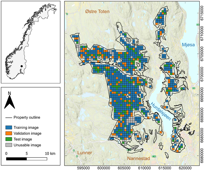
Fig. 1. Map of the forests of Mathiesen Eidsvold Værk ANS located in Akershus County, Norway. The area was divided into images tiles of 512 m × 512 m.
2.2 Datasets
In this study, three primary datasets were utilized: multispectral aerial images, ALS data, and a stand map created by an expert interpreter with 30 years of experience. These datasets form the foundation of the U-Net modelling process for delineating forest stands. The aerial images provide spectral information, the ALS data supports the construction of a CHM, and the reference data serves as the basis for creating masks for training and validating the model.
The multispectral aerial images were obtained from Norway’s national aerial image database (https://www.norgeibilder.no/). Under Norway’s national aerial image acquisition program, images are captured every 5–10 years, depending on the type of area (Norwegian Mapping Authority 2024), and are stored in the database as orthophotos. The images used in the current study were acquired on three different dates, August 13th, August 14th, and September 1st, 2022, from an altitude of 6300 m above ground level. The images contain four color channels – red, green, blue, and near-infrared – with a spatial resolution of 0.25 m, and an 8-bit radiometric resolution.
ALS data was collected on July 17th, 2021, as part of the forest management planning inventory. A dual channel Riegl VQ 1560II was flown at 3500 m above ground level, with a pulse repetition rate of 250 kHz per channel, a scan rate of 56 lines per second, and a 20% lateral overlap between lines. The resulting pulse density was 1.4 pulses m–2.
In DL, the term “ground truth” typically refers to the data used for model training and evaluation. However, this poorly reflects the highly subjective nature of stand delineation and the interpretive process of creating maps (Magnusson et al. 2007). Therefore, the manually delineated stands are referred to as “reference data”.
The reference data comprised a stand map of 13 000 stands, manually delineated by an expert interpreter with 30 years of experience using photogrammetry and a CHM constructed from the ALS data as support (Table 1). Each stand was classified as either forest or non-forest. The forest stands were further attributed with additional information, such as species composition, age, site index, and stand development stage. Development stage was determined based on age, species, and site index. Stage I includes bare forest land, while Stage II represents recently regenerated forest with trees up to 8–9 m in height. Stage III is designated for young production forests, Stage IV for old production forests, and Stage V for mature forests (Eid et al. 1987). This division aids forest managers in making informed decisions regarding silvicultural treatments. Stage I represents forests in need of regeneration, while Stage II indicates areas where pre-commercial thinning should be considered. Stages III and IV are young and old thinning-phase forests, and Stage V consists of mature forests ready for harvest. These development stages served as the basis for creating reference masks used in model training and evaluation.
| Table 1. Forest stand characteristics from the stand database created during the 2021 forest management planning inventory. | |||||||||||
| Class1 | Stands (n) | Area (ha) | Mean age | Volume (%) | Lorey’s mean height (m) | ||||||
| Spruce | Pine | Broadleaves | Min | Max | Mean | ||||||
| NF | 3079 | 5159 | - | - | - | - | - | - | - | ||
| I | 260 | 538 | 0 | - | - | - | 0.0 | 22.0 | 0.4 | ||
| II | 1966 | 4799 | 15 | - | - | - | 0.1 | 20.0 | 2.3 | ||
| III | 2828 | 10 803 | 44 | 90 | 2 | 8 | 5.1 | 23.3 | 13.4 | ||
| IV | 2302 | 6563 | 68 | 89 | 2 | 9 | 6.5 | 25.4 | 16.2 | ||
| V | 2889 | 7938 | 101 | 91 | 3 | 6 | 6.4 | 28.5 | 18.7 | ||
| 1 NF – non-forest, I-V – stand development stages. | |||||||||||
2.3 Pre-processing
Before segmentation can be performed, the data must undergo several preprocessing steps to ensure consistency and compatibility with the U-Net model. This section describes the preparation of the aerial imagery and ALS data. Additional steps, including tiling, data cleaning, normalization, and the division of the data into training, validation and test set, are also outlined. Furthermore, the reference data used for modelling and evaluation, along with data augmentation techniques designed to enhance model robustness, are discussed. Together, these steps establish a dataset that is well-suited for segmentation.
When applying a U-Net-based segmentation model, a choice must be made regarding the spatial resolution of the image. An image with a finer spatial resolution provides the model with more detailed information but also requires longer processing time and larger memory usage. Additionally, with pixel-wise predictions, the spatial resolution of the image will affect the precision of the final delineation. Based on preliminary tests, a 1-m resolution was considered a suitable compromise between the level of information contained in the images, processing time, and the precision of stand boundaries produced by the model. Thus, the original 0.25-m resolution was downsampled to 1 m by averaging groups of 16 pixels.
A CHM was constructed from the ALS data using the lidR v. 4.1.2 package (Roussel et al. 2020; Roussel and Auty 2024) in R (R Core Team 2023). It was created at a 1-m spatial resolution to match the aerial images and align with the previously mentioned considerations. The CHM was then incorporated as an additional channel to the aerial images, resulting in a five-layer raster composite.
The raster composite was too large to fit into memory, and the model requires consistently sized image tiles. To address this, the raster composite was divided into tiles measuring 512 m × 512 m, producing individual 5-channel images of 512 × 512 pixels. Any images extending beyond the forest property boundaries were discarded to avoid issues with missing values. After this filtering, 809 images were retained. They were then visually inspected for discrepancies caused by the one-year time difference between the ALS and aerial image acquisitions. Twenty-eight images were excluded because the aerial images showed clear-cuts not present in the CHM; however, minor discrepancies were permitted to avoid excluding an excessive number of images. Furthermore, images covering protected areas with missing delineations were removed. After these exclusions, 760 images were retained for analysis.
These images were randomly split into training (70%, 532 images), validation (15%, 114 images), and test (15%, 114 images) sets. All images were normalized to a range of [0, 1] by dividing each pixel in the spectral layers by 255, and each pixel in the CHM by 39, which corresponds to the largest observed value in the CHM.
The U-Net model expects input in raster format, thus, to use the stand database as reference data for the model, the vector data was first rasterized based on the development stage of the forest. Due to the similarity of the stand development stages I and II, these stages had to be combined. Typically, a stand is moved from development stage I to development stage II when the regeneration is deemed satisfactory, usually after planting. However, these plants are not visible in the spectral data and the CHM, necessitating the merging of development stage I and II. Ultimately, the raster layer representing the reference stands consisted of five classes: four based on development stages – Class I-II, Class III, Class IV, and Class V – and a single class for non-forested areas, Class NF. The raster was then one-hot encoded, a process that involves converting each class into a separate binary layer, with pixel values 1 indicating presence and 0indicating absence of the corresponding class. This process created a five-layer raster, with one layer per class, referred to as masks. The distribution of the classes across the three datasets used for analysis is shown in Fig. 2.
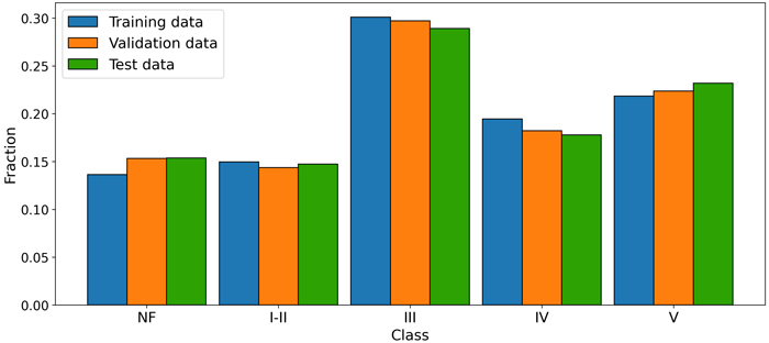
Fig. 2. Fraction of pixels across the five classes (NF – non-forest, I-II – V development stages) for each of the datasets used in model development and evaluation.
Training DL models requires large and diverse datasets to ensure that the model learns effectively and can generalize well to new, unseen data (Barbedo 2018). Data augmentation, which involves modifying the appearance of images, is a technique used to artificially expand training datasets and improve performance in real-world applications (Goodfellow et al. 2016). In this study, common augmentation techniques, including horizontal flipping (Xu et al. 2023), brightness and contrast adjustments (Xiao et al. 2024) and Gaussian-noise addition (Moradi et al. 2020) were applied during model training, meaning the images were automatically altered between training epochs.
Shadows can affect the accuracy of the border placement between clear-cuts and mature forests (Næsset 1998). Shadow length and orientation appeared broadly consistent across the imagery, and horizontal flipping was applied to account for natural variation in shadow orientation. This technique effectively reverses shadow orientation.
Brightness and contrast were adjusted with ±10% to simulate different lighting conditions. This value was chosen based on visual inspection and testing. This range ensured realistic representation without overly dark or bright outputs that could impair learning.
Gaussian noise was added to the images to reduce the model’s reliance on fine detail, helping the model to learn more robust features and improve generalization (Sietsma and Dow 1991). A zero-centered Gaussian distribution with a 0.1 standard deviation was used to balance challenge and realism, avoiding overly noisy images.
Initial tests helped determine the values of the augmentations discussed above. Smaller values tended to stabilize model convergence during later training stages, while larger values negatively impacted overall performance. Additionally, given the high-quality nature of the commercial aerial images from the national database, which are under strict quality control, there is minimal need to alter their appearance substantially, as the model is expected to encounter similarly high-quality images in real-world applications.
2.4 Model architecture
In this study, the general architecture of the U-Net (Ronneberger et al. 2015) was applied with slight adaptations. The model architecture is depicted in Fig. 3, and the subsequent sections outline the key architectural components and modifications, including batch normalization, pooling operations, dropout regularization, weight initialization, activation functions, and the choice of loss function. These elements were carefully chosen to enhance the model’s performance for stand delineation.
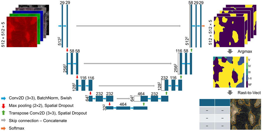
Fig. 3. Model architecture and flow of images through the model. Each blue box represents multi-channel feature maps produced by the model. The numbers along the vertical axis indicate the spatial dimensions of the images. The number of channels in the feature maps are denoted by the number on top of each box (Ronneberger et al. 2015).
During training, the distribution of activations in DL models can shift as the parameters of previous layers update (Ioffe and Szegedy 2015). Batch normalization mitigates this issue through normalization of layer inputs to have zero mean and unit variance. This leads to improved training stability and faster model convergence. Consequently, batch normalization was implemented in the model.
Pooling operations were performed by using 2 × 2 max-pooling with a stride of 2. This procedure selects the strongest response within each 2 × 2 region of the feature maps produced by the convolutional layers. Selecting the strongest responses introduces robustness by retaining dominant features against noise and small variations (Raschka and Mirjalili 2019; Matoba et al. 2022). Pooling also reduces the dimensionality of the feature maps, resulting in faster and more efficient calculations. Additionally, polling enables deeper layers to aggregate information over a larger spatial context, improving the model’s ability to recognize patterns across varying positions (Nirthika et al. 2022).
In DL, a neuron refers to a computational unit within a neural network that processes input data and passes its output to subsequent layers. Dropping neurons in a procedure known as dropout is a common way to regularize neural networks as this reduces overfitting by preventing the model from relying too much on specific features. However, in convolutional layers, standard dropout is less effective because the surrounding pixels are spatially correlated, meaning that dropping individual neurons does not sufficiently disrupt learned patterns. For this reason, 2D spatial dropout, as proposed by Tompson et al. (2015), was applied to achieve regularization by dropping entire feature maps.
The initialization of weights is important for model performance. If weights are initialized with too small values it can lead to the gradients vanishing when the errors are propagated through the model layers, slowing down or halting the learning process. If the weights are set too large, the gradients can grow exponentially leading to exploding gradients. This causes unstable updates of model weights, which in turn results in unstable learning and poor performance. To address these issues, the initialization technique proposed by He et al. (2015) was applied. This technique draws the initial weights from a truncated normal distribution whose variance is scaled according to the incoming connections of each layer. By maintaining a stable variance of the activations as data propagates through the network, the initialization effectively reduces the risk of vanishing or exploding gradients.
Activation functions are used after convolutional layers to introduce non-linearity into the U-Net model. The original U-Net architecture used the ReLU activation function between convolutional layers. However, an alternative activation that closely resembles the ReLU function, known as Swish has emerged, with findings indicating that it could outperform ReLU (Ramachandran et al. 2017). Initial tests comparing ReLU and Swish revealed that Swish tended to perform slightly better for the task and data in this study. Consequently, Swish was selected for implementation after each convolutional layer.
For the final layer, the softmax function was applied. This function outputs a vector with a length equal to the number of classes in the dataset, where each number represents the probability of a pixel belonging to a specific class. These probabilities sum to 1 and the pixel is assigned to the class with the largest probability.
Based on initial experimentation with several loss functions, a loss function based on the Tversky index (Eq. 1), known as the focal Tversky loss (Eq. 2) demonstrated the best performance, producing coherent polygons with minimal noise or graininess. The Tversky index accounts for true positives (TP), false positives (FP), and false negatives (FN), with the parameters α and β adjusting the weighting of FP and FN, respectively. Building on this formulation, Abraham and Khan (2019) proposed the focal Tversky loss, which computes the Tversky index independently for each class and averages the results over classes (N). Additionally, a focal parameter (γ) affects the impact of different training examples, which can help mitigate effects of class imbalance (Abraham and Khan 2019).


2.5 Implementation and training
The model was implemented using the Keras API with TensorFlow backend and trained on a NVIDIA RTX 8000 GPU with 48GB of memory and CUDA capabilities.
Models were trained for up to 80 epochs, using a batch size of 16 and shuffling the data between epochs. Hyperparameter optimization was performed using Optuna’s hyperparameter optimization framework (Akiba et al. 2019). Experiments were tracked using Weights & Biases (Biewald 2020), a tool for logging training metrics, visualizing performance, and automatically saving model weights. In total, 200 instances of the model were trained and evaluated using this setup.
A search space was defined for key hyperparameters, as outlined in Table 2. The search space included model parameters such as the number of filters, filter size, learning rate, and dropout rate. Additionally, the alpha, beta, and gamma parameters of the focal Tversky loss function were optimized using Optuna.
| Table 2. Hyperparameters and search intervals as input to Optuna. | ||
| Hyperparameter | Data type | Interval |
| Model parameters | ||
| Number of filters | Int | [8, 32] |
| Filter size | Int | [3, 7] |
| Learning rate | Float | [0.00001, 0.001] |
| Dropout rate | Float | [0.0, 0.5] |
| Loss parameters | ||
| Alpha | Float | [0.3, 0.7] |
| Beta | Float | 1 – alpha |
| Gamma | Float | [1, 3] |
A pruning strategy using Optuna’s median pruner was implemented to streamline the hyperparameter optimization. To help achieve this, the first 10 trials were set to run without pruning to establish a baseline. Pruning was then applied to all subsequent trials. The first 30 epochs of each trial were allowed to run without pruning to ensure that models initially performing poorly due to random weight initialization had sufficient time to improve. After the initial 30 epochs, a model was pruned if its performance fell below the median of all previous trials.
2.6 Evaluation criteria
Model evaluation is essential in the training and implementation of DL models, enabling the assessment of model performance during both training and final evaluation. Quantifying agreement between the predicted mask and reference mask was achieved through calculating a population confusion matrix for the final predictions on the test data (Olofsson et al. 2014). The matrix systematically compares reference classes with predicted classes and includes four key outcomes: true positives (TP), true negatives (TN), false positives (FP), and false negatives (FN). Due to the large number of pixels, the confusion matrix was normalized by dividing each cell by the total pixel count, so each cell represents a proportion relative to the overall total.
Overall accuracy was calculated as the proportion of correct predictions relative to all predictions (Eq. 3).

To provide a more nuanced evaluation, producer’s accuracy (PA; Eq. 4) and user’s accuracy (UA; Eq. 5) were calculated for each class. Producer’s accuracy is the ratio between TP and the number of reference pixels in that class (TP + FN), reflecting the models omission errors. User’s accuracy measures the ratio between the number of TP for a class and the total number of predicted pixels in that class (TP + FP), indicating commission errors. Producer’s and user’s accuracy are also commonly known as recall and precision, respectively, in machine learning applications.


For unbalanced datasets the accuracy metric tends to give biased estimates. In unbalanced datasets the model will get a large accuracy value simply by predicting the majority class. Another reliable metric for binary classification tasks is the Mathews correlation coefficient (Eq. 6; MCC) (Matthews 1975). MCC considers all correctly (TP, TN) and incorrectly (FP, FN) classified instances. The MCC metric ranges from –1 to 1, where –1 indicates all instances being incorrectly classified, 0indicates random predictions, and 1 represents perfect classification. MCC is widely regarded as a reliable and robust metric for binary classification tasks (Chicco and Jurman 2023).

To extend MCC to multiclass classification, the metric was calculated individually for each class and then averaged across all classes (N) – a process known as macro averaging. Macro averaging ensures that all classes are weighted equally, regardless of their relative abundance, which is important when all classes are considered equally important in the evaluation. This extended metric is referred to as mMCC (Eq. 7).

Because of the nature of the delineation process and the fact that the reference data represents only a single realization, the evaluation process cannot fully rely on metrics derived from the confusion matrix. While large values for the accuracy or mMCC metric would suggest good performance, small boundary discrepancies inevitably introduce misclassified pixels. Moreover, as the reference represents only one of many possible versions, these discrepancies do not always indicate actual errors.
The confusion matrix treats all correctly and incorrectly classified pixels uniformly. However, the reality is more nuanced. For instance, a pixel predicted as Class IV but belonging to Class III is arguably less misclassified than if it belonged to Class II, as the former represents a smaller deviation. In other words, the degree of error varies depending on how close the actual class is to the predicted class.
To gain a more detailed understanding of how the model handles the complexities of different stand boundaries, the images were inspected visually. Three representative examples displaying key characteristics of the model predictions were selected and are presented in the results section. Example 1 was selected to demonstrate close agreement between the manual interpretation and model prediction, and to illustrate the role of the CHM. Example 2 was selected to show a case with strong agreement in boundary placement, but differing class assignments. Example 3 was selected to highlight a limitation of the model in capturing contextual and operational conditions that in some cases resulted in stands not suitable as separate units.
3 Results
3.1 Tuning and the final model
The training loss decreased consistently, showing that the model was successfully minimizing the error on the training set. The validation loss closely followed the training loss throughout the training process, with no clear signs of overfitting (Fig. 4a). The model balanced the alpha and beta parameters of the focal Tversky loss function and applied a value of 1.3 for the focal parameter (γ). Additionally, the model applied 3 × 3 filters, with 29 filters in the initial layer (Fig. 3). This configuration achieved maximum validation mMCC (Fig. 4b) and accuracy values (Fig. 4c) of 0.64 and 0.73, respectively, after 73 epochs, and was automatically saved by Weights & Biases at this stage. When evaluated on the test data, the U-Net model achieved mMCC and accuracy values of 0.63 and 0.72.
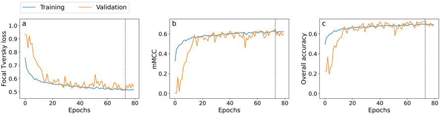
Fig. 4. Training history for the best performing model, showing development of the focal Tversky loss, mMCC, and overall accuracy for both training (blue) and validation (orange) data over 80 epochs. A dotted vertical line marks the best epoch, at which the model was automatically saved by Weights & Biases.
A more in-depth look at the tuning process revealed that models with smaller filters (3 × 3) tended to outperform models utilizing larger filters (5 × 5 and 7 × 7). Plotting the results of some models using larger filters showed a tendency to produce maps with less noise, but at the cost of more inaccurate boundaries.
3.2 Classification and confusion matrix
The model demonstrated strong performance for Class NF and Class I-II, with UA values of 85% and 84% and PA values of 78% and 75%, respectively. Indicating that the model correctly classified a large proportion of pixels in these classes (Table 3). The largest source of error for these classes was misclassification as Class III (young thinning-phase forest), though misclassification rates to other classes were relatively low.
| Table 3. Normalized confusion matrix comparing the predicted mask with the reference masks in the test data. Each cell gives the proportion relative to the total number of pixels being evaluated. The detected and correctly classified pixels (TP) are represented by the bold elements along the diagonal of the shaded area. Producer’s accuracy (PA) and user’s accuracy (UA) are calculated for each class, giving insights into omission and commission errors. | ||||||||
| Reference | Sum | UA | ||||||
| NF | I-II | III | IV | V | ||||
| Predicted | NF | 0.12 | 0.00 | 0.01 | 0.01 | 0.01 | 0.14 | 0.85 |
| I-II | 0.00 | 0.11 | 0.01 | 0.00 | 0.00 | 0.13 | 0.84 | |
| III | 0.02 | 0.02 | 0.21 | 0.03 | 0.01 | 0.29 | 0.73 | |
| IV | 0.00 | 0.00 | 0.05 | 0.10 | 0.02 | 0.18 | 0.55 | |
| V | 0.01 | 0.01 | 0.01 | 0.05 | 0.18 | 0.26 | 0.70 | |
| Sum | 0.15 | 0.15 | 0.29 | 0.18 | 0.23 | 1 | ||
| PA | 0.78 | 0.75 | 0.73 | 0.55 | 0.79 | |||
Class III also showed great accuracy, with PA and UA values of 73%, effectively balancing commission and omission errors. The main errors for this class were confusion with Class IV (old thinning-phase forest), as indicated by the relatively large misclassification rates between the two classes.
Class IV proved particularly challenging for the model, achieving substantially smaller UA and PA values than the other classes (Table 3). Similarly to Class III, Class IV showed a balance between UA and PA, indicating that predictions for this class were also balanced between omission and commission errors. The primary source of confusion was classification as either Class III or Class V (forest ready for harvest), with Class V being the largest source of confusion.
Class V had the lowest rate of omission errors, with a PA of 79%. However, the UA value for Class V was notably smaller than the PA, indicating that commission errors were a larger issue. This was primarily caused by confusion with Class IV.
3.3 Visual interpretation and boundary accuracy
Applying the model to the test data showed a fast inference time of just 20 seconds for the entire test dataset, demonstrating an ability to greatly reduce the time consumption for stand delineation.
Visual inspection of the boundaries produced by the model revealed promising results. Example 1 (Fig. 5) displays the model’s prediction and reference for a single image tile. The figure demonstrates that the model can accurately recreate the boundaries defined by the manual interpreter. Close visual inspection of the clear-cut boundaries shows that the model effectively captures the nuances and intricacies of these edges.
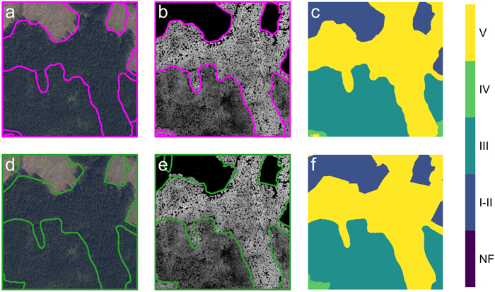
Fig. 5. Model prediction and corresponding reference data for Example 1. (a-c) Model prediction results: (a) delineated boundaries overlaid on the RGB image, (b) boundaries overlaid on the canopy height model, and (c) predicted classification mask. (d-f) Reference data: (d) annotated boundaries overlaid on the RGB image, (e) boundaries overlaid on the canopy height model, and (f) reference classification mask. Class labels: NF – non-forest, I-II - V – development stage.
Comparing the clear-cut boundaries reveals a discrepancy in border location between the aerial images and CHM. Notably, both the reference and predicted boundaries align with the CHM. Similar results, where the boundaries most closely resemble the CHM, were observed across other images and classes. For instance, the model shows comparable behavior in delineating forest roads adjacent to mature forests, where tree shadows obscure the edges in images but remain clear in the CHM, potentially indicating a higher reliance on the CHM for accurate delineations.
Example 2 (Fig. 6) showcases another important aspect of the model predictions. There is good agreement in the overall boundary placement of the stands. However, there are a few misclassified stands (stands 1 and 2), and the model has combined two stands (stands 3 and 4) into a single large stand. According to the forest management plan, stands 1 and 2 are 44 and 43 years old, respectively, and both stands have the same site index value. Based on the definition of the development stages, the lower age limit for classifying these stands as Class IV is 45 years. Therefore, if the age given in the forest management plan is assumed correct, stands 1 and 2 are only one and two years away from qualifying as Class IV, meaning the model’s predictions could be considered accurate. Additionally, since the aerial images were acquired one year after the forest management plan was created, stand 2 would already have reached Class IV at the time of image acquisition.
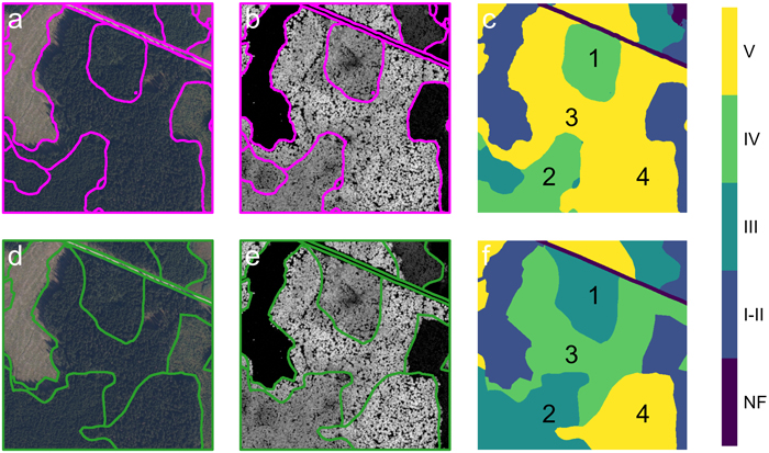
Fig. 6. Model prediction and corresponding reference data for Example 2. (a-c) Model prediction results: (a) predicted boundaries overlaid on the RGB image, (b) boundaries overlaid on the canopy height model, and (c) predicted classification mask. (d-f) Reference data: (d) annotated boundaries overlaid on the RGB image, (e) boundaries overlaid on the canopy height model, and (f) reference classification mask. Class labels: NF – non-forest, I-II - V – development stage. Numbered regions (1-4) highlights classification nuances: regions 1 and 2 show stands with ages near the transition between classes III and IV; regions 3 and 4 show where the model has merged two neighboring stands into a single operational unit.
Comparing the forest management plan inventory and the model predictions, stands 3 and 4 appear similar (Table 4). For stand 3 the lower age limit for Class V is 70 years, while the reported age is 67 years, indicating it’s close to reaching the predicted class. This similarity suggests that, in terms of forest stand definition, the two stands are homogenous and could be treated as a single operational unit for silvicultural treatment. The goal of delineation is to create operational units, supporting the model’s decision to combine these areas.
| Table 4. Stand characteristics for stands 3 and 4. | ||
| Attribute | Stand 3 | Stand 4 |
| Class | IV | V |
| Age | 67 | 82 |
| Site index (H40) | G20 | G20 |
| Tree species composition1 (S, P, B) | (99, 0, 1) | (100, 0, 0) |
| Volume (m3 ha–1) | 462.0 | 497.2 |
| Height (m) | 23.6 | 24.5 |
| Basal area (m2 ha–1) | 46 | 48 |
| Mean diameter (cm) | 26.3 | 27.4 |
| 1 Percentage distribution of spruce (S), pine (P), and broadleaves (B) | ||
Stand delineation requires considering the entire scene in its context, which poses a challenge for the model. As seen in Example 3 (Fig. 7), the model treats a small stand in the top center as a separate unit within the peatland, while the manual interpreter connects it to a nearby stand with similar characteristics. Only considering forest characteristics, the model’s boundaries are more accurate, as the manual interpreter includes peatland. However, as the delineation process aims to define operational units, and the smaller stand is too small to function as a separate unit, it is logical to connect the two stands. This pattern is observable across multiple images, where the model separates small regions based on forest characteristics but doesn’t account for operational requirements.
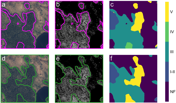
Fig. 7. Model prediction and corresponding reference data for Example 2. (a-c) Model prediction results: (a) predicted boundaries overlaid on the RGB image, (b) boundaries overlaid on the canopy height model, and (c) predicted classification mask. (d-f) Reference data: (d) annotated boundaries overlaid on the RGB image, (e) boundaries overlaid on the canopy height model, and (f) reference classification mask. Class labels: NF – non-forest, I-II - V – development stage.
Another notable fact in Example 3 is found in the center of the image. The manual interpreter has extended the boundary leftward compared to the model. There is no clearly defined boundary in this region of the image; instead, there is a gradual transition in characteristics, with the stand characteristics of the adjacent stand differing only slightly.
4 Discussion
The model demonstrates solid performance, effectively aligning with the general trends of the reference dataset. The mMCC and overall accuracy indicate strong agreement between the predicted and reference mask for the test data. The results highlight the model’s ability to generalize effectively within the forest property subject to analysis in this study, which is characterized by intensive silvicultural practices, minimal variability in tree species composition – primarily pure spruce forests – and clear stand structure. Additionally, the proposed DL framework offers rapid inference time, substantially reducing the time and cost associated with manual interpretation. This efficiency is promising for computational scalability to large-scale operational forestry, where implementation of a tiling strategy could enable the production of continuous stand maps (Huang et al. 2018).
Importantly, operational scalability due to rapid inference time does not imply transferability across differing forest structures or management regimes. While the well managed forests forming the basis of this study facilitate strong model performance, they limit generalizability of the findings to less managed forests. For instance, Diedershagen et al. (2004) observed that their automated framework for delineation based on CHM performed worse in structurally heterogenous forest, and was unable to make distinctions between adjacent stands comprising different tree species.
The current study utilized a relatively small dataset of only a few hundred images. While U-Net has demonstrated success with small datasets in certain applications (Ronneberger et al. 2015), these results often depend on highly controlled conditions. In contrast, stand delineation is subjective and frequently produced under time pressure, introducing variability that may not be well-captured by the current dataset. Further testing across diverse forest types and stand structures using a larger dataset is necessary to confirm the model’s generalizability and ensure robustness.
Expanding the dataset to include a broader range of forest conditions, management practices, and phenological stages would likely enhance the model’s performance and its applicability to more diverse contexts. The study found that the model relied heavily on the CHM, potentially due to the structural information in the CHM being particularly important for delineation. However, the one-year time discrepancy between the ALS data and aerial images complicates this interpretation. Another possibility is that this reliance stems from better agreement between the ALS-derived CHM and the reference data. Future work could address this limitation by constructing the CHM using point clouds from digital photogrammetry, ensuring temporal consistency with the aerial images.
Another notable source of discrepancy is the model’s difficulty with stand boundaries between stands of similar characteristics. This effect would likely also be observed between different interpreters in manual interpretation, but this is not testable in the current study as only the product of a single interpreter is available. Alternatively, the issue could stem from the model lacking sufficient contextual information to make informed decisions. For example, forestry operations are influenced by terrain properties, as they determine accessibility, harvesting feasibility, and operational efficiency (Berg 1981; Silversides and Sundberg 1989). In Norway, systems for terrain classification have been made and applied to define operational units (Norwegian Agricultural University 1970; Samset 1975). Manual interpreters often rely on terrain features, such as ridges, valleys, and slopes, to delineate stand boundaries in a way that align with operational requirements. However, this information was absent from the provided model inputs. Incorporating terrain indices, derived from a digital terrain model, could potentially improve the model’s ability to delineate boundaries in complex cases and produce outputs that are more in line with operational needs.
The Classes IV and V proved difficult to segment and this led to substantial misclassification issues, suggesting challenges in distinguishing these classes, potentially caused by overlapping feature characteristics. However, after discussing these findings with the expert interpreter it was revealed that this is likely a semantic issue. The instructions used for delineation during the 2021 forest management inventory did not strictly follow the class definitions given by Norwegian Agricultural University (1970) in all cases, leading to inconsistencies. A similar conclusion was drawn by Tiede et al. (2004) who found that misclassification was primarily related to semantic issues in class definitions, linked to the underlying mapping guidelines.
While the current results are promising, there remains considerable room for improvement. Adaptations of U-Net, incorporating more complex architectures, have demonstrated potential for enhanced performance. For example, combinations with residual networks (Diakogiannis et al. 2020) can help build deeper networks extracting hierarchical features, while inception modules (Cahall et al. 2019) capture features across multiple scales. Implementing attention gates (Oktay et al. 2018) can help the model focus on the most relevant aspects of an image. These strategies have shown to improve segmentation accuracy in other applications, and future research could incorporate these strategies for stand delineation.
As noted by Pukkala (2021), different criteria can guide the delineation process, making direct comparisons between methods challenging. Recent advancements in automated procedures for stand delineation have demonstrated the ability to produce stands that are more internally homogenous compared to manual interpretations (Pukkala et al. 2024; Xiong et al. 2024). However, this is not always the main goal of the delineation process. Historical and cultural silvicultural traditions, along with local conditions, also represent an important frame for the delineation process. Importantly, stands also function as operational units. In this context DL frameworks could be especially useful, as they try to replicate the decisions of the manual interpreter while accommodating the unique criteria, traditions, and local conditions that influence the delineation process.
The definition of “ground truth” poses a key challenge in this study. While the model shows good agreement with the reference dataset, the subjectivity inherent in its creation introduces potential biases. Several factors impact the quality of the reference data, including the limited number of acquisition dates, which restricts the data variability. Spectral signatures change in accordance with phenological changes and can produce quite different impressions depending on the time of acquisition. Additionally, handling spatial data introduces inherent correlations. Despite splitting the dataset into training, validation, and test sets, and excluding the test set during training, nearby images remain spatially correlated. The entire property is also managed under a single silvicultural regime, and the three datasets are all derived from the same ALS and aerial image acquisitions. These factors combined can limit the generalizability of the model. To fully exploit the strengths of DL methods and make models capable of accounting for all aspects of the delineation process, it is essential to extend the dataset to incorporate data from different areas and multiple interpreters. This would improve the robustness of the reference data by capturing a broader range of expert perspectives and delineation conditions, enabling the model to account for all aspects of the delineation process.
5 Conclusion
This study presents a novel approach to automated stand delineation and has shown great potential for the implementation of DL algorithms. The model, based on the U-Net architecture, demonstrates strong potential for automating stand delineation in well managed forest environments, aligning well with the reference data and offering substantial efficiency improvements over manual methods. However, its application to more complex and heterogenous forest conditions remains untested, and further research is needed to enhance generalizability. Expanding the dataset, integrating additional data types, improving the alignment of the input data, and exploring more advanced architecture will be essential to improve performance and ensuring that the model can handle diverse forest conditions and different delineation criteria. Ultimately, while the model is a promising step towards automating stand delineation using DL, future work must address the challenges of variability, data complexity, and the subjective nature of “ground-truth” to maximize its applicability and robustness in real-world applications.
Declaration of openness of research materials, data, and code
The airborne laser scanning data and the stand map are owned by the forest owner, the aerial images are owned by the Norwegian Mapping Authority and the authors do not have permission to share the data. Code used in the study is openly available in GitHub repository: https://github.com/haksandu/semantic_segmentation_of_forest_stands_using_deep_learning.
Acknowledgements
We sincerely thank Ngoc Huynh Bao from the Norwegian University of Life Sciences for help getting started with the U-Net model, Mathiesen Eidsvold Værk ANS for providing data, and Viken Skog SA for preparation of data.
Authors’ contributions
Håkon Næss Sandum: Conceptualization, Methodology, Visualization, Validation, Writing – original draft; Oliver Tomic: Conceptualization, Supervision, Writing – review and editing; Hans Ole Ørka: Conceptualization, Supervision, Writing – review and editing; Erik Næsset: Funding acquisition, Writing – review and editing; Terje Gobakken: Conceptualization, Funding acquisition, Project administration, Supervision, Writing – review and editing.
Disclosure statement
The authors declare that they have no known competing financial interests or personal relationships that could have appeared to influence the work reported in this paper.
Funding sources
This work was supported by the Center for Research-based Innovation SmartForest: Bringing Industry 4.0 to the Norwegian forest sector (NFR SFI project no. 309671, smartforest.no).
References
Abraham N, Khan NM (2019) A novel focal tversky loss function with improved attention u-net for lesion segmentation. 16th International Symposium on Biomedical Imaging (ISBI 2019), Venice, Italy, pp 683–687. IEEE. https://doi.org/10.1109/ISBI.2019.8759329.
Akiba T, Sano S, Yanase T, Otha T, Koyama M (2019) Optuna: a next-generation hyperparameter optimization framework. Proceedings of the 25th ACM SIGKDD International Conference on Knowledge Discovery & Data Mining, New York, NY, USA, pp 2623–2631. Association for Computing Machinery. https://doi.org/10.1145/3292500.3330701.
Andrews G (1934) Air survey and forestry: developments in Germany. For Chron 10: 91–107. https://doi.org/10.5558/tfc10091-2.
Axelson H, Nilsson B (1993) Skoglig flygbildstolkning. [Forest aerial image interpretation]. In: Minell H (ed) Flygbildsteknik og fjärranalys. Skogsstyrelsen, pp 295–336.
Baatz M, Schäpe A (2000) Multiresolution segmentation: an optimization approach for high quality multi-scale image segmentation. In: Strobl J, Blaschke T, Griesbner G (eds) Proceedings of Angewandte Geographische Informationsverarbeitung 12: 12–23. Wichmann Verlag, Karlsruhe, Germany.
Baker FS (1950) Principles of silviculture. McGraw-Hill. ISBN 9780070033856.
Barbedo JGA (2018) Impact of dataset size and variety on the effectiveness of deep learning and transfer learning for plant disease classification. Comput Electron Agric 153: 46–53. https://doi.org/10.1016/j.compag.2018.08.013.
Berg S (1981) Terrain classification for forestry in the nordic countries. In: Laban P (ed) Proceedings of IUFRO/ISSS Workshop on Land Evaluation for Forestry. International Institute for Land Reclamation and Improvement /ILRI, Wageningen, Netherlands, pp 152–166.
Bhatnagar S, Gill L, Ghosh B (2020) Drone image segmentation using machine and deep learning for mapping raised bog vegetation communities. Remote Sens 12, article id 2602. https://doi.org/10.3390/rs12162602.
Bhatnagar S, Puliti S, Talbot B, Heppelmann J B, Breidenbach J, Astrup R (2022) Mapping wheel-ruts from timber harvesting operations using deep learning techniques in drone imagery. For 95: 698–710. https://doi.org/10.1093/forestry/cpac023.
Biewald L (2020) Experiment tracking with weights and biases. wandb.com.
Cahall DE, Rasool G, Bouaynaya NC, Fathallah-Shaykh HM (2019) Inception modules enhance brain tumor segmentation. Front Comput Neurosci 13, article id 14. https://doi.org/10.3389/fncom.2019.00044.
Chicco D, Jurman G (2023) The Matthews correlation coefficient (MCC) should replace the ROC AUC as the standard metric for assessing binary classification. BioData Min 16, article id 4. https://doi.org/10.1186/s13040-023-00322-4.
De Groeve T, Lowell K (2001) Boundary uncertainty assessment from a single forest-type map. Photogramm Eng Remote Sens 67: 717–726.
Dechesne C, Mallet C, Le Bris A, Gouet-Brunet V (2017) Semantic segmentation of forest stands of pure species combining airborne lidar data and very high resolution multispectral imagery. ISPRS J of Photogramm Remote Sens 126: 129–145. https://doi.org/10.1016/j.isprsjprs.2017.02.011.
Diakogiannis FI, Waldner F, Caccetta P, Wu C (2020) ResUNet-a: a deep learning framework for semantic segmentation of remotely sensed data. ISPRS J of Photogramm Remote Sens 162: 94–114. https://doi.org/10.1016/j.isprsjprs.2020.01.013.
Diedershagen O, Koch B, Weinacker H (2004) Automatic segmentation and characterisation of forest stand parameters using airborne lidar data, multispectral and fogis data. Int Arch Photogramm Remote Sens and Spatial Inf Sci 36: 208–212. https://www.isprs.org/proceedings/xxxvi/8-w2/DIEDERSHAGEN.pdf. Accessed 30 October 2024.
Eid T, Nersten S, Svendsrud A, Veidahl A (1987) Handbok for planlegging i skogbruket. [Handbook for planning in forestry]. Landbruksforlaget.
Eysn L, Hollaus M, Schadauer K, Pfeifer N (2012) Forest delineation based on airborne LIDAR data. Remote Sens 4: 762–783. https://doi.org/10.3390/rs4030762.
Goodfellow I, Bengio Y, Courville A (2016) Dataset augmentation. In: Goodfellow I, Bengio Y, Courville A (eds) Deep learning. MIT Press, pp 236–238. ISBN 0262035618. https://www.deeplearningbook.org/contents/regularization.html. Accessed 30 October 2024.
He K, Zhang X, Ren S, Sun J (2015) Delving deep into rectifiers: surpassing human-level performance on imagenet classification. Proceedings of IEEE International Conference on Computer Vision (ICCV), Santiago, Chile, pp 1026–1034. https://doi.org/10.1109/ICCV.2015.123.
Hernando A, Tiede D, Albrecht F, Lang S (2012) Spatial and thematic assessment of object-based forest stand delineation using an OFA-matrix. Int J Appl Earth Obs Geoinf 19: 214–225. https://doi.org/10.1016/j.jag.2012.05.007.
Huang B, Reichman D, Collins L M, Bradbury K, Malof J M (2018) Tiling and stitching segmentation output for remote sensing: basic challenges and recommendations. arXiv 1805.12219. [Preprint]. https://doi.org/10.48550/arXiv.1805.12219.
Husch B, Miller CI, Beers TW (1993) Forest mensuration, 3rd edition. Krieger Publishing Company. ISBN 978-0894648212.
Ioffe S, Szegedy C (2015) Batch normalization: accelerating deep network training by reducing internal covariate shift. Proceedings of the 32nd International Conference on Machine Learning, Lille, France. PMLR 37: 448–456. https://proceedings.mlr.press/v37/ioffe15.html. Accessed 30 October 2024.
Kentsch S, Lopez Caceres ML, Serrano D, Roure F, Diez Y (2020) Computer vision and deep learning techniques for the analysis of drone-acquired forest images, a transfer learning study. Remote Sens 12, article id 1287. https://doi.org/10.3390/rs12081287.
Koch B, Straub C, Dees M, Wang Y, Weinacker H (2009) Airborne laser data for stand delineation and information extraction. Int J Remote Sens 30: 935–963. https://doi.org/10.1080/01431160802395284.
Leckie DG, Gougeon FA, Walsworth N, Paradine D (2003) Stand delineation and composition estimation using semi-automated individual tree crown analysis. Remote Sens. Environ 85: 355–369. https://doi.org/10.1016/S0034-4257(03)00013-0.
Løvli Ø (2022) Landskapsplan for Mathiesen Eidsvold Værk ANS. [Landscape plan for Mathiesen Eidsvold Værk ANS]. https://www.mev.no/skogen/milj%C3%B8sertifisering. Accessed 30.10.2024.
Magnusson M, Fransson JE, Olsson H (2007) Aerial photo-interpretation using Z/I DMC images for estimation of forest variables. Scand J For Res 22: 254–266. https://doi.org/10.1080/02827580701262964.
Matoba K, Dimitriadis N, Fleuret F (2022) The theoretical expressiveness of maxpooling. arXiv 2203.01016 530-531. [Preprint]. https://doi.org/10.48550/arXiv.2203.01016.
Matthews BW (1975) Comparison of the predicted and observed secondary structure of T4 phage lysozyme. Biochim Biophys Acta Protein Struct 405: 442–451. https://doi.org/10.1016/0005-2795(75)90109-9.
Moradi R, Berangi R, Minaei B (2020) A survey on regularization strategies for deep models. Artif Intell Rev 53: 3947–3986. https://doi.org/10.1007/s10462-019-09784-7.
Mustonen J, Packalen P, Kangas A (2008) Automatic segmentation of forest stands using a canopy height model and aerial photography. Scand J of For Res 23: 534–545. https://doi.org/10.1080/02827580802552446.
Næsset E (1998) Positional accuracy of boundaries between clearcuts and mature forest stands delineated by means of aerial photointerpretation. Can J For Res 28: 368–374. https://doi.org/10.1139/x97-221.
Næsset E (1999a) Assessing the effect of erroneous placement of forest stand boundaries on the estimated area of individual stands. Scand J For Res 14: 175–181. https://doi.org/10.1080/02827589950152908.
Næsset E (1999b) Effects of delineation errors in forest stand boundaries on estimated area and timber volumes. Scand J For Res 14: 558–566. https://doi.org/10.1080/02827589908540821.
Næsset E (2014) Area-based inventory in Norway – from innovation to an operational reality. In: Maltamo M, Næsset E, Vauhkonen J (eds) Forestry applications of airborne laser scanning: concepts and case studies. Springer Netherlands, pp 215–240. https://doi.org/10.1007/978-94-017-8663-8_11.
Nantel J (1993) A new and improved digitizing method based on the Thiessen (Voronoi) algorithm. Proceedings Sixth Annual Genasys International Users Conference, Fort Collins, Colorado, pp 12–25.
Nirthika R, Manivannan S, Ramanan A, Wang R (2022) Pooling in convolutional neural networks for medical image analysis: a survey and an empirical study. Neural Comput Appl 34: 5321–5347. https://doi.org/10.1007/s00521-022-06953-8.
Norwegian Agricultural University (1970) D – Arealinndeling og bestandsutforming. [Spatial division and stand design]. In: Handbok for planlegging i skogbruket. [Handbook for Planning in Forestry].
Norwegian Mapping Authority (2024) Program for omløpsfotografering. https://www.kartverket.no/geodataarbeid/program-for-omlopsfotografering. Kartverket. Accessed 30 October 2024.
Oktay O, Schlemper J, Folgoc LL, Lee M, Heinrich M, Misawa K, Mori K, McDonagh S, Hammerla NY, Kainz B (2018) Attention u-net: learning where to look for the pancreas. arXiv 1804.03999. [Preprint]. https://doi.org/10.48550/arXiv.1804.03999.
Olofsson P, Foody GM, Herold M, Stehman SV, Woodcock CE, Wulder MA (2014) Good practices for estimating area and assessing accuracy of land change. Remote Sens Env 148: 42–57. https://doi.org/10.1016/j.rse.2014.02.015.
Pukkala T (2021) Can Kohonen networks delineate forest stands? Scand J For Res 36: 198–209. https://doi.org/10.1080/02827581.2021.1897668.
Pukkala T, Aquilué N, Kutchartt E, Trasobares A (2024) A hybrid method for delineating homogeneous forest segments from LiDAR data in Catalonia (Spain). Eur J Remote Sens 57, article id 2425337. https://doi.org/10.1080/22797254.2024.2425337.
R Core Team (2023) R: a language and environment for statistical computing. R Found for Statistical Comp. https://www.R-project.org/. Accessed 30 October 2024.
Ramachandran P, Zoph B, Le QV (2017) Searching for activation functions. arXiv 1710.05941. [Preprint]. https://doi.org/10.48550/arXiv.1710.05941.
Raschka S, Mirjalili V (2019) Python machine learning, 3rd edition. Packt. ISBN 9781789955750.
Ronneberger O, Fischer P, Brox T (2015) U-net: convolutional networks for biomedical image segmentation. In: Navab N, Hornegger J, Wells W, Frangi A (eds) Medical Image Computing and Computer-Assisted Intervention (MICCAI 2015). Lecture Notes in Computer Science 9351. Springer, Cham, pp 234–241. https://doi.org/10.1007/978-3-319-24574-4_28.
Roussel J-R, Auty D (2024) Airborne LiDAR data manipulation and visualization for forestry applications, version 4.2.3. https://cran.r-project.org/package=lidR. Accessed 30 October 2024.
Roussel J-R, Auty D, Coops NC, Tompalski P, Goodbody TRH, Meador AS, Bourdon J-F, de Boissieu F, Achim A (2020) lidR: an R package for analysis of Airborne Laser Scanning (ALS) data. Remote Sens Env 251, article id 112061. https://doi.org/10.1016/j.rse.2020.112061.
Samset I (1975) Skogterrengets tilgjengelighet og terrengforholdenes innflytelse på skogtilstanden i Norge. [The accessibility of forest terrain and its influence on forestry conditions in Norway]. Meddr Nor Inst Skogforsk 32: 1–92. ISBN 82-7169-029-9.
Schiefer F, Kattenborn T, Frick A, Frey J, Schall P, Koch B, Schmidtlein S (2020) Mapping forest tree species in high resolution UAV-based RGB-imagery by means of convolutional neural networks. ISPRS J Photogramm Remote Sens 170: 205–215. https://doi.org/10.1016/j.isprsjprs.2020.10.015.
Sietsma J, Dow RJF (1991) Creating artificial neural networks that generalize. Neural Netw 4: 67–79. https://doi.org/10.1016/0893-6080(91)90033-2.
Silversides CR, Sundberg U (1989) Operational efficiency in forestry, vol. 2: practice. Kluwer Academic Publishers. https://doi.org/10.1007/978-94-017-0506-6.
Smith DM (1986) The practice of silviculture, 8th edition. John Wiley & Sons. ISBN 978-0471800200.
Tiede D, Blaschke T, Heurich M (2004) Object-based semi automatic mapping of forest stands with laser scanner and multi-spectral data. Int Arch Photogramm Remote Sens Spat Inf Sci 36: 328–333.
Tompson J, Goroshin R, Jain A, LeCun Y, Bregler C (2015) Efficient object localization using convolutional networks. Proceedings of IEEE Conference on Computer Vision and Pattern Recognition (CVPR), Boston, MA, USA, pp 648–656. https://doi.org/10.1109/CVPR.2015.7298664.
Trimble Germany GmbH (2021) Trimble documentation: eCognition Developer 10.1 reference book.
Xiao J, Guo W, Liu J (2024) Exploring data augmentation effects on a singular illumination distribution dataset with ColorJitter. 3rd International Conference on Image Processing and Media Computing (ICIPMC), Hefei, China, pp 75–81. IEEE. https://doi.org/10.1109/ICIPMC62364.2024.10586593.
Xiong H, Pang Y, Jia W, Bai Y (2024) Forest stand delineation using airborne LiDAR and hyperspectral data. Silva Fenn 58, article id 23014. https://doi.org/10.14214/sf.23014.
Xu M, Yoon S, Fuentes A, Park DS (2023) A comprehensive survey of image augmentation techniques for deep learning. Pattern Recognit 137, article id 109347. https://doi.org/10.1016/j.patcog.2023.109347.
Total of 63 references.
