Riku Tarvainen  ,
Kirsi Riekki,
Heikki Ovaskainen,
Asko Poikela,
Kalle Kärhä,
Jukka Malinen
,
Kirsi Riekki,
Heikki Ovaskainen,
Asko Poikela,
Kalle Kärhä,
Jukka Malinen
Estimating stand variables in first-thinnings using harvester data
Tarvainen R., Riekki K., Ovaskainen H., Poikela A., Kärhä K., Malinen J. (2025). Estimating stand variables in first-thinnings using harvester data. Silva Fennica vol. 59 no. 3 article id 25014. https://doi.org/10.14214/sf.25014
Highlights
- The idea was to identify the trees removed from the strip roads from the harvester data and use them as a sample of the initial growing stock of the first thinning stand
- The goal was also to estimate the number of stems, basal area and diameter distribution of the growing stock after thinning
- The sampling method based on identifying strip road trees is applicable to monitoring the density of the remaining growing stock at first thinning stands.
Abstract
First thinning is an important operation in forest management because it determines the further growth of the whole stand. Harvester operators open strip roads to the thinning stand and select which trees are removed and which are left to grow. Modern cut-to-length harvesters produce precise information about the dimensions and positions of the cut trees. The location of the harvester is already commonly recorded to harvester production (hpr) files, according to the StanForD 2010 standard, and recording the position of the harvester head is also becoming more common. The aim of this study was to develop a method to estimate the stem count and basal area of the remaining growing stock using this novel harvester data. Precision hpr data from Komatsu harvesters and reference field measurements were gathered from seven stands in western Finland in the summer of 2024. In the method used, the strip road trees were identified and used as samples representing the initial growing stock. The remaining growing stock was estimated using diameter distributions, and by subtracting the harvested trees from the initial growing stock. The results were evaluated using Reynold’s error index, in addition to a visual interpretation of the diameter distributions with respect to the reference data. We found that the method had the potential to determine the basal area and diameter distribution of the remaining growing stock. In the future, this method can be automated, which will allow automated reporting and quality management in first-thinning operations.
Keywords
forest inventory;
diameter distribution;
stand variables;
harvester data;
accurate GNSS positioning;
harvesting quality;
Reynold’s error index
-
Tarvainen,
Metsäteho Oy, Vernissakatu 1, FI-01300 Vantaa, Finland
 https://orcid.org/0009-0001-2336-3125
E-mail
riku.tarvainen@metsateho.fi
https://orcid.org/0009-0001-2336-3125
E-mail
riku.tarvainen@metsateho.fi
-
Riekki,
Metsäteho Oy, Vernissakatu 1, FI-01300 Vantaa, Finland
https://orcid.org/0009-0007-8366-3297
E-mail
kirsi.riekki@metsateho.fi
-
Ovaskainen,
Metsäteho Oy, Vernissakatu 1, FI-01300 Vantaa, Finland
https://orcid.org/0000-0001-5063-6662
E-mail
heikki.ovaskainen@metsateho.fi
- Poikela, Metsäteho Oy, Vernissakatu 1, FI-01300 Vantaa, Finland E-mail asko.poikela@metsateho.fi
- Kärhä, University of Eastern Finland, School of Forest Sciences, Faculty of Science, Forestry and Technology, P.O. Box 111, FI-80101 Joensuu, Finland E-mail kalle.karha@uef.fi
-
Malinen,
Metsäteho Oy, Vernissakatu 1, FI-01300 Vantaa, Finland
https://orcid.org/0000-0002-5023-1056
E-mail
jukka.malinen@metsateho.fi
Received 30 April 2025 Accepted 13 December 2025 Published 22 December 2025
Views 17543
Available at https://doi.org/10.14214/sf.25014 | Download PDF

Supplementary Files
1 Introduction
In forest management, first thinning is the first commercial harvesting operation after forest regeneration. It is crucial for the subsequent forest rotation period, the primary goal typically being to remove lower-quality trees and leave the ones with the most potential to grow. For example, in Finland, first thinning is recommended in Scots pine (Pinus sylvestris L., hereafter referred to as pine), Norway spruce (Picea abies (L.) Karst., hereafter referred to as spruce), and birch (Betula spp.) forests when the dominant tree heights reach 13–16 m, the recommended density being 700–1300 trees ha–1 after thinning (Tapio Oy 2025). In Finland, around 150 000 ha of first thinnings are harvested annually.
Due to the significance of first thinnings for the future forest development, the quality of the thinning is essential. One aspect of good thinning quality is ensuring that the variables of the remaining growing stock after thinning, particularly stand density, basal area per hectare and crown metrics, comply with general forest management recommendations. Having stand variables available after the thinning operation enables their use in, for example, self-monitoring of the work and quality reporting. In this work, growing stock means trees on a stand, which have commercial value.
A common way to describe growing stock is by determining its diameter distribution (Hyink 1983; Kilkki 1989). The diameter distribution involves the number of trees in specific diameter classes. This distribution is useful for assessing the silvicultural state of a forest because it allows for calculating the variables of the entire growing stock. Additionally, it facilitates the simulation of individual tree growth and the estimation of timber assortment volumes (Kangas 2003; Vähä-Konka et al. 2025).
The diameter distribution can be obtained using various methods. Manual diameter measurements are accurate, but labour-intensive and time-consuming, making them impractical for large forest areas. Parametric distribution functions, such as the Weibull or beta functions, rely on the parameter prediction of a theoretical model (Lee 2021). Alternatively, non-parametric methods, such as a k-nearest-neighbor search from an existing database of forest stands, have been shown to predict diameter distributions more accurately (Maltamo 1998, 2018; Peuhkurinen 2018).
Obtaining some of the stand variables accurately using remote sensing methods is challenging. There are several possible manual and automated approaches for performing laser scanning of forests (Fassnacht et al. 2024; Gollob et al. 2020), but manual alternatives are not cost-effective for nation-wide scanning. Aerial laser scanning (ALS), which can cover large areas quickly, has a low temporal resolution and does not penetrate the forest canopy effectively for example, to directly determine tree diameters (Kangas et al. 2019). Therefore, in ALS, tree diameters are modeled based on tree heights, and tree variables are currently determined as areal averages of sample plots. In ALS-based individual tree detection, roughly 80% or less of the trees are detected, corresponding to the accuracy of the stem count, and the root mean square error (RMSE) for diameters at breast height (DBH) vary between approximately 10 and 20% (Hyyppä et al. 2024; Muhojoki et al. 2024).
In Finland, the inventory of growing stock is currently produced by the Finnish Forest Centre (FFC), which is the authority responsible for collecting data on forest variables, usage, harvesting results, and forest nature features. Forest resource information is openly and freely accessible at both the stand and 16 × 16-m-grid level (Finnish Forest Centre 2025a). The FFC’s forest data is derived from a combination of manual reference sample plot measurements, laser scanning in six-year cycles, and aerial photography (Finnish Forest Centre 2025b). The accuracy of this information varies depending on the method.
For ALS, the accuracy requirements for the sample plots specify a maximum RMSE of 15–30% for DBH and 20–45% for basal area and volume. Additionally, for eight out of 10 compartments, the average diameter can vary by a maximum of 3 cm and the total volume by 20%. In manual reference measurements, the error margin for the total volume of tree stock typically varies between 15 and 25%. Between laser surveys, only stand-level forest variables are updated computationally, often using, for example, growth models (FFC 2023a, 2023b).
Although the forest inventory data in Finland is rather advanced, more-accurate information would improve the quality reporting of thinning operations. The interval between laser surveys is too long for reporting growing stock variables for self-monitoring purposes, for example. The forest data includes average forest variables, but diameter distributions are not available. The accuracy of forest variables is generally lower in younger and mixed forests––that is, forests that are typically subject to first thinning (FFC 2023b). Therefore, simply determining the remaining growing stock by subtracting harvested trees from the open forest data before thinning involves quite large inaccuracies.
As described above, obtaining accurate variables of the growing stock after thinning can be challenging when using manual or remotely sensed data. An alternative approach is to use the data that harvesters already measure and record during thinning (Räsänen et al. 2019). Harvester data are recorded in harvester production (hpr) files according to the forest machine StanForD 2010 standard (Skogforsk 2025). These hpr files contain information about harvested trees, including accurate measurements of their commercial length, diameters, species, and volume.
Modern harvesters can also collect the location data of both the harvester and, in some cases, the harvester head at the moment of the felling cut. The position of the harvester head in relation to the harvester can be calculated geometrically using the bearing of the harvester, the boom angle in relation to the base machine front frame, and the length of the boom, all of which can be recorded in the hpr files.
The positioning accuracy of harvesters varies, ranging from a few meters up to nine meters when using a recreational-level Global Navigation Satellite System (GNSS) receiver (Kaartinen et al. 2015). In addition, the location of modern harvesters equipped with real-time kinematic (RTK) correction for GNSS positioning can be determined much more precisely, typically within 0.5 m, under forest canopy (Hannrup and Möller 2022; Cho et al. 2024).
In general, the position of the harvester head can be determined with good accuracy in relation to the harvester because it is measured using sensors on the boom joints. The boom can typically extend up to 11 m. Ideally, the position of the harvester head will correspond to the location of the felled tree. In practice, determining this position requires accounting for the detailed geometry of the boom and harvester head as well as the radius of the felled tree.
The accuracy of harvester head positioning relative to field references has been investigated in previous studies and depends strongly on system configuration. In Taipale et al. (2022), where a recreational-grade GNSS receiver was used on the harvester and the boom length was measured without sensors on the extension boom, the average position accuracy of the harvester head was 3.9 m. However, achieving this result required numerical filtering of the harvester location and bearing. By contrast, Hannrup and Möller (2022) found that a Komatsu harvester head equipped with RTK-corrected GNSS positioning and a complete measurement of the harvester head position achieved an accuracy of 0.56 m. Another study with a similar harvester configuration reported an accuracy of 0.54 m and a standard deviation of 0.41 m when comparing harvester head positions to reference measurements (Ylä-Pöntinen et al. 2025). In addition, Hannrup and Möller (2025) examined the accuracy of Ponsse’s RTK-corrected GNSS positioning and reported an accuracy of 0.49 m, with variation ranging between 12 and 90 cm.
In the quality reporting of first thinnings, harvester data can be used to determine the forest variables of the remaining growing stock after thinning. All the trees on the strip roads have to be removed to enable harvesting with forest machines. The method relies on identifying all the trees removed from the strip roads using the harvester head position to estimate the initial growing stock before thinning. The remaining growing stock is then estimated by subtracting all the cut trees from the initial growing stock. Because the area of the opened strip roads is typically approximately 20% of the total harvested area, the removed trees provide a reasonably representative sample. The accuracy of the method depends on correctly identifying the strip road trees and their precise growing area.
Skogforsk has developed and tested the method described above (Bhuiyan et al. 2016), with the basal area weighted diameter being estimated based on the strip road trees. In this method, the strip road tree selection was performed using hpr data, based on the harvester boom angle. Trees felled within a boom angle of ±30° are classified as strip road trees. In Bhuiyan et al. (2016), 83% of manually recorded strip road trees were correctly identified in the hpr data. In addition, the identified strip road trees had a smaller average diameter than the average diameter in the stand. Because boom length measurements were not employed, some trees felled outside the strip road area may have been misclassified, and some trees within the strip road area may have been excluded. Including boom length measurements would be expected to improve the accuracy of the method.
To address the discrepancy in estimated stem counts, Skogforsk’s method was refined (Hannrup et al. 2015). In the refined method, the stem count was corrected using a thinning quotient, which is a scaling factor between the diameter of the basal area weighted mean tree and the basal area weighted mean diameter. Thinning quotients for different tree species are determined using existing stand data from forest owner companies, which is obtained via laser scanning. By applying this correction to determine the variables of the remaining growing stock from hpr data, the systematic deviation (i.e., bias) in estimated measurement area -wise stem counts and basal areas was reduced to less than 2.2%. The standard deviation of the measurement area -wise basal area estimates after first thinning was 2.2 m2 ha–1 (13%), with deviations for individual stands ranging between approximately ±5 m2 ha–1 (Hannrup et al. 2015). The refined method calculates the results, when the hpr file is input into the program code during the thinning operation. Harvester operators have found this method useful because it reduces the number of stands where thinning was overly strong with respect to the recommended thinning guidelines (Burström 2016).
The approach described above relates to determining the variables of the remaining growing stock after the thinning operation has been completed. However, from a quality perspective, harvester data is most beneficial in ensuring that the recommended thinning intensity has been achieved during the operation. Providing real-time assistance for harvester operators is a long-term goal in developing automated methods based on harvester data (Lindroos et al. 2015; Lopatin et al. 2023). This can be achieved by giving harvester operators information about the remaining growing stock during the thinning operation. Accurate data on harvester head positions allows provision of the information needed for such a detailed, real-time follow-up of the stand variables while the thinning operation is ongoing. Therefore, it is important to first manage the stand-level estimation after thinning to then be able to shift toward the real-time estimation.
The objective of this study was to estimate the remaining stem count, diameter distribution, and average basal area of a thinned stand using only hpr files after first-thinning operations. The strip road trees were identified using boom angle and length and then using these as samples of the initial growing stock. The diameter distributions after thinning were then estimated and compared to reference measurements, and the basal areas were calculated.
2 Material and methods
2.1 Harvester data
The harvester hpr data were from first-thinning cuttings in the municipalities of Sastamala and Teuva in western Finland from seven separate stands, each representing thinning operations in managed forests. The cuttings were performed in January–July 2024 by two Komatsu 901XC-6 harvesters with C93 harvester head and an 11m boom reach. The hpr files contained the accurate location and bearing of the harvester, the boom angle and length, and the tree species and dimensions of each felled tree. The accurate locations of the harvesters were determined using the Komatsu MaxiFleet Precision feature, which uses the Global Navigation Satellite System (GNSS), and RTK correction. The RTK correction requires reference points where correction signal is received and virtual reference station service where correction is computed (Kaartinen et al. 2024).
The tree-wise coordinates of the harvester and the parameters of the harvester boom were recorded every time the felling cut was made. The data were extracted from the hpr files and inserted into a relational database. The data were then exported into the Geographical Information System program QGIS 3.28.9 (QGIS Development Team 2025). The harvester data were originally recorded in the WGS84 (EPSG:4326) coordinate system and were then reprojected into ETRS-TM35FIN (EPSG:3067) in QGIS.
The strip road network lengths were calculated using the method developed by Metsäteho Oy (Ovaskainen and Riekki 2022), in which the locations of the harvester base machine were used to generate the computational strip road network. The geographical locations of the harvester head, representing the locations of the harvested trees, were calculated directly based on the harvester’s geometry, using the harvester’s location and the position of the boom in relation to the harvester.
The DBHs of the harvested trees were calculated from the log diameters measured by the harvester. In the harvester measurements, the diameter representing the DBH was commonly measured at a constant height of 120 cm from the felling cut, instead of 130 cm from the ground. This originates from assuming that the height of the felled tree’s stump is 10 cm. In cases where the stump was more than 10 cm tall, the diameter would be too small because it would have been measured above the correct breast height. For each tree, the diameters were transformed into ideal taper curves using Metsäteho’s in-house tool (Supplementary file S1), which uses least-squares fitting and the model from Laasasenaho (1982). The total height of each tree was estimated during the fitting process. The DBH of the stem from the ground was calculated from the fitted taper curve.
2.2 Measurement areas and field reference data
In the harvested first-thinning stands, measurement areas of approximately 1 ha were established in QGIS program. Measurement areas were used both to estimate the variables of the remaining trees from harvester data and to perform reference measurements of the remaining trees at the site. The objective for each area was to provide a representative sample of the stand and include a balanced strip road layout with more than two parallel strip roads. The borders of the areas were delineated to obtain a relatively straightforward strip road network rather than a highly curved one (Fig. 1). A straightforward strip road network had direct strip roads to the same main direction over the measurement area, whereas a curvy strip road network involved more crossings and turns. In addition, felled trees were required on both sides of the strip roads at approximately crane-length distance.
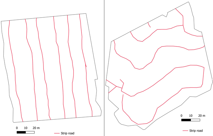
Fig. 1. On the left, an example of a straightforward and on the right, an example of a curvy strip road network on the measurement area.
The tree-wise field reference data were collected at the measurement areas during the summer of 2024, a few months after the thinning operations. For all measurement areas every tree with a DBH of over 45 mm, the DBH was measured with measuring scissors, the tree species was identified, and the position was recorded by placing a measuring stick at the base of the tree. The tree position information was not used in this study, except for ensuring that the tree was located within the measurement area. Each measured tree was also classified as normal, dead, wounded, snapped, or multi-topped. The stand variables of the measurement areas are presented in Table 1.
| Table 1. Stand variables from the measurement areas. These include the total length of the strip road per hectare after thinning, main tree species, and shape description of the strip road network. | |||||
| Measurement area ID | Area, ha | Municipality | Strip road density, m ha–1 | Main tree species | Strip road network shape |
| A | 0.7 | Teuva | 589 | Spruce | Curvy |
| B | 1.2 | Sastamala | 610 | Pine | Straightforward |
| C | 1.0 | Sastamala | 522 | Pine | Curvy |
| D | 1.0 | Teuva | 533 | Pine | Straightforward |
| E | 0.9 | Sastamala | 488 | Pine | Curvy |
| F | 1.2 | Teuva | 436 | Pine | Straightforward |
| G | 0.8 | Teuva | 536 | Pine | Straightforward |
| Mean | 1.0 | 531 | |||
The position data were measured using a Trimble R12i GNSS receiver and Trimble Access field measuring software (Trimble, Sunnyvale, CA, USA). The measurement uncertainty of the receiver was limited to 0.05 m both horizontally and vertically. The GNSS receiver was mounted at a height of 1.5 m on top of a mapping stick. Real-time kinematic positioning and an inertial measurement unit were used in determining the position. The RTK corrections were obtained through Trimble’s network service.
Additionally, the locations of the strip roads were recorded from each measurement area by walking along the strip roads’ middle lines with the same GNSS receiver. It is noteworthy that these location data were not used in estimating the growing stock, but only in alternative approach for validating the main results. Using the strip road lines’ geographical locations, the specific strip road width and the tree location information in the hpr file, a tree data could be extracted from the hpr file to calculate reference values (Supp. file S2).
2.3 Strip road trees
The strip road trees were defined as those trees cut in front of the harvester from a zone of harvester’s width. The method to extract strip road trees from the hpr file was solely based on the boom angle and length in relation to the harvester front frame at the moment of felling cut. The geographical locations of the harvester or the manually field-recorded strip roads were not used in identifying the strip road trees.
To identify the strip road trees, transverse distances to the left or right in relation to the middle line of the harvester front frame were calculated for all harvester head locations. Here, it was assumed that the middle line of the harvester front frame corresponded to the middle line of the strip road on the measurement area, in other words the harvester was assumed to drive in the middle of the strip road. The strip road trees were extracted from each hpr file corresponding to the specific measurement area.
When compiling a distance distribution, the strip road trees were expected to peak symmetrically at the center of the distribution. The width of the Komatsu harvesters used in this study was approximately 2.8 m (Komatsu 2024). When using tracks on the harvester, the width increased to 3.0 m. Additionally, the harvester head position was assumed to correspond to the center point of the harvested tree. In those cases where trees were growing at the edges of the harvester track zone, the center point of a tree could lie outside the zone, while the cross-section of the tree could lie partly inside the zone. In practice, such trees would be classified as strip road trees by taking the radii of the edge trees into account in determining the zone width. Therefore, a zone width of 3.2 m was used for the strip road identification using the positions of the harvester head (Fig. 2a).
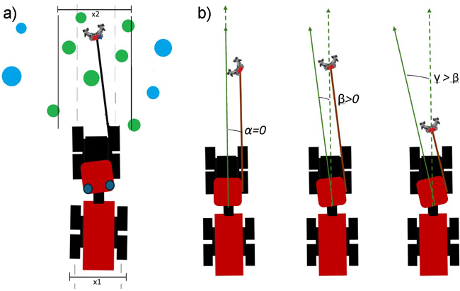
Fig. 2. a) Illustration showing identification of the strip road trees. Here, x1 is the width of the harvester (2.8 m) and x2 is the width of the strip road zone (3.2 m). b) Illustration showing how asymmetry in the Komatsu harvester affects the boom angle. The angles α, β and γ show the angle between the boom and the middle line of the harvester’s front frame and demonstrate how this angle changes when the harvester’s head is moved in relation to the middle line of the harvester.
By analyzing the distance distribution of all the cut trees, a sideways bias in the peak of the distribution was recognized. In Komatsu harvesters, the boom is placed on the right side of the cabin, and this asymmetry affected the tree positions relative to the harvester by causing a small, but systematic, bias. When the tree was directly in front of the harvester at the middle line, the recorded boom angle was not zero because the boom had to have been turned to the left (Fig. 2b). The bias increased the closer the tree was to the harvester. This bias was corrected using Eq. 1.

where BoomAngleCorr is the corrected angle of the boom at the moment of felling cut, BoomAngle is the angle of the boom at the moment of felling cut, dt is the transverse distance of the boom base from the middle line of the harvester, and BoomExtension is the length of the boom at the moment of felling cut.
Here, dt = 0.4 m was used. The corrected distance distribution of the felled trees (Fig. 3) was practically symmetrical with respect to the middle line of the harvester. Due to the bias correction, the geographical locations of the harvester head had to be re-determined.

Fig. 3. Distance distribution of all harvested stems, showing the distance from the middle line of the harvester. Substantially higher frequency close to the middle line of the harvester demonstrates our method to identify strip road trees.
The strip road trees were then identified based on the corrected distance values. The zone width used in the identification was 3.2 m, which corresponds to the width of the harvester, the harvester tracks, and the tree diameters at the edge of the strip road zone (Fig. 3). The distance distribution accords with this width because the number of felled trees decreased substantially when the distance exceeded 1.6 m from the middle line of the harvester (Fig. 3).
2.4 Diameter distributions
After identifying the strip road trees, as described above, the diameter distributions for estimating the remaining growing stock were compiled. The remaining growing stock was estimated by assuming that the strip road trees represented the initial growing stock of the whole measurement area before the thinning operation. Then, all the harvested trees were subtracted from the assumed initial growing stock (Fig. 4). All these calculations were performed using hectare-wise diameter distributions with 10-mm classes of DBHs. Only those trees with DBHs of at least 70 mm were included in the diameter distributions.

Fig. 4. The workflow of the estimation method outlines the calculation steps of diameter distributions and to estimate hectare-wise growing stock after thinning.
The diameter distributions for both the strip road trees and all the harvested trees were compiled separately. The diameter distribution of the initial growing stock was calculated from the distribution of the strip road trees by hectare-wise scaling with the area of the strip road. This area required information on the strip road length and was calculated from the computed strip road network. Hence, multiplying the strip road length by the strip road width (a width of 2.9 m was used) resulted in the area of the strip road. The width was selected so that the number of trees per hectare corresponded to the reference values.
All the harvested trees data included both the strip road trees and the trees that were harvested from the area between the strip roads. Similarly to the above, the diameter distribution of all the harvested trees was scaled hectare-wise by the area of the measurement area because all the harvested trees were removed from the area of the whole measurement area.
The reference data for the initial growing stock was compiled by adding all harvested trees and measured standing trees together to form one dataset. The reference diameter distribution of the initial growing stock before the operation was formed as explained above, using the whole measurement area in hectare-wise scaling. The geographical locations of the harvester head were needed to identify all the harvested trees located within the area of the measurement area.
The first analysis of the diameter distributions was to compare the initial growing stock determined from the strip road trees with the corresponding reference growing stock. The second analysis was to compare the estimated diameter distribution of the remaining growing stock with the distribution of measured reference trees after thinning. In the estimation of the distribution of the remaining growing stock, the distribution of all harvested trees was subtracted from the estimated distribution of the initial growing stock in each class. If the class-wise subtraction resulted in a value less than zero, a zero value was used.
The hectare-wise stem count and basal area were calculated for each dataset and for each measurement area. The stem count was calculated by adding the numbers of observations in each diameter class. In calculating the basal area, the diameter of each tree in each diameter class was estimated to be the mean value of the class. For example, in the 150–160 mm diameter class, the diameter of all the trees was estimated as 155 mm. The measurement area -wise basal area was then calculated by adding all the diameter-class-wise basal areas together.
Statistical tests, like Kolmogorov-Smirnov test (Kolmogorov 1933; Massey 1951) in a comparison of diameter distributions, were considered, but the results were not interpreted further since the statistical tests are not always reasonable for large sample sizes. With large datasets, even minor differences between distributions become statistically significant, which consistently leads to rejection of the null hypothesis without providing meaningful information about the practical relevance of the differences (Eriksson and Lindroos, 2014). Therefore, to compare the estimated and reference distributions, Reynold’s error index, Rg (Reynolds et al. 1988) was calculated using Eq. 2.
![]()
where n is the index of the diameter class, N is the index of the largest diameter class in the datasets, gn is the basal area of the diameter class n, xn is the stem count of the diameter class n of the estimated distribution, and yn is the stem count of the diameter class n of the reference distribution. In interpreting Reynold’s error index, lower values represent a good fit of the similarity of distributions. An absolute value of the difference of each class is weighted by the basal area, which reflects the correspondence of the distributions, especially at large diameters. Therefore, differences in large diameters affect the value of Reynold’s error index more than differences in smaller diameters.
2.5 Estimation of uncertainties
The uncertainties of the hectare-wise stem count and basal area were evaluated by using the propagation of uncertainties (Taylor 1982). The main sources of the measurement uncertainties considered in this analysis were the uncertainties of the GNSS position of the trees before thinning, and the uncertainties of the stem diameters. The position uncertainty of the trees affected the stem count, since near the boundaries of the measurement areas the stems within area can be incorrectly laying outside, or vice versa. The position uncertainty was mainly governed by the GNSS positioning inaccuracy of the hpr stems – the uncertainties of the field recorded positions with high accuracy GNSS receiver were small in comparison to those of the hpr stems. It is noteworthy, that the uncertainty of the GNSS positions of the stems does not affect the identification of the strip road trees, which was done only based on the boom parameters in relation to the harvester. The uncertainties of the boom length and angle were assumed small with respect to the other uncertainties.
The effect of the uncertainty of the stem positions on the hectare-wise stem count before thinning, ΔN, was taken into account by calculating the relative area of the zone of uncertainty around the measurement area. The area of the measurement area A was assumed constant. Then, the uncertainty of the stem count was calculated from Eq. 3, which was derived by using the propagation of uncertainties:
![]()
where N is the number of stems of hpr data within the measurement area, wuz = 0.54 m is the width of the zone of uncertainty, which was the mean accuracy of the hpr stems when compared to the field references (Ylä-Pöntinen et al. 2025), and LA is the perimeter of the measurement area. This uncertainty ΔN was further propagated for the classes of the diameter distributions ΔNn by their relative proportions.
Regarding the uncertainties of the stem diameter, they were assumed to originate mainly from two separate sources. Firstly, the taper curve fitting caused uncertainties to the fitted DBH values, denoted as Δdf,n. Despite being overall rather small, they were included into this analysis, because the diameter-wise standard deviations of the fitted taper curves were available from the validation of the fitting results (Suppl. file S1). Secondly, in compiling the diameter distributions, the diameters were divided into 10-mm classes, and the middle points of the classes were used in further calculations. For example, all trees of the class 110−120 mm were assumed to have a diameter of 115 mm. This caused a rounding error between −5 to +5 mm, and within one class the diameters were assumed to be uniformly distributed. Therefore, the standard deviation of rounding is Δdr = 5 mm /![]() for each diameter class. The direct measurement uncertainties of the diameters by harvester and field recording were assumed small in comparison to the uncertainties described above.
for each diameter class. The direct measurement uncertainties of the diameters by harvester and field recording were assumed small in comparison to the uncertainties described above.
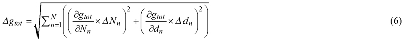
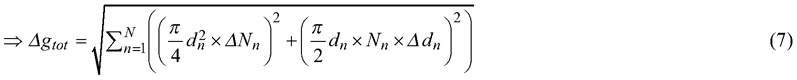
In calculating the basal area, both the uncertainties of the stem counts and the diameters were taken into account by the propagation of uncertainties. The total basal area gtot is summed from the diameter-class wise basal areas, presented using variables dn and Nn in Eq. 4:

Calculating first-order expansion of Taylor series of gtot gives Eq. 5:

where gn,0 is constant. Then, the uncertainty of the basal area Δgtot is obtained from the variance (Δgtot)2, assuming that the diameter class -wise variables dn and Nn are independent (Eqs. 6−8):
![]()
3 Results
The estimates and references for the hectare-wise stem count and basal area before thinning are presented in Table 2. The estimated stem count before thinning varied between the measurement areas. In five measurement areas, the estimated stem count was higher than the reference stem count, with the relative differences ranging between 2 and 14%. However, the numerical results indicate that the relative basal area differences were consistently lower than the stem count differences.
| Table 2. Description of measurement areas before first thinning. The table contains measurement areas, their strip road densities and the numerically estimated stem counts and basal areas based on our method. In addition, reference values are shown, as well as their relative differences. | ||||||
| Measurement area ID | Estimated stem count, N ha–1 | Reference stem count, N ha–1 | Diff-% | Estimated basal area, m2 ha–1 | Reference basal area, m2 ha–1 | Diff-% |
| A | 1596 | 1641 | –2.7 | 22.0 | 24.4 | –10.0 |
| B | 1369 | 1203 | 13.8 | 17.4 | 16.2 | 7.5 |
| C | 1749 | 1671 | 4.7 | 24.1 | 24.9 | –3.2 |
| D | 1586 | 1602 | –1.0 | 22.0 | 24.4 | –9.6 |
| E | 1399 | 1376 | 1.7 | 22.4 | 24.1 | –7.0 |
| F | 1500 | 1363 | 10.1 | 22.2 | 22.0 | 0.9 |
| G | 2016 | 1771 | 13.8 | 27.1 | 26.6 | 1.7 |
| Mean | 1602 | 1518 | 5.5 | 22.5 | 23.2 | –3.3 |
The relative differences between the estimated and reference stem counts after thinning varied substantially, ranging from approximately –24 to +30% (Table 3). However, the estimated stem counts differed similarly before and after thinning, except in measurement area E, where the estimated difference in the stem count before thinning was 1.7% higher, becoming measurably lower (–9.9%) after thinning compared to the references. For all measurement areas, substantial differences were calculated for basal area after thinning. The estimated basal areas varied from approximately –29 to +13% compared to the reference values.
| Table 3. Description of numerical results of measurement areas after first thinning. Estimated stem counts, basal areas based on our method presented earlier in this paper. In addition, reference values, and their relative differences are shown. | ||||||
| Measurement area ID | Estimated stem count, N ha–1 | Reference stem count, N ha–1 | Diff-% | Estimated basal area, m2 ha–1 | Reference basal area, m2 ha–1 | Diff-% |
| A | 770 | 1016 | –24.2 | 12.6 | 17.8 | –29.1 |
| B | 720 | 552 | 30.4 | 10.3 | 9.1 | 13.1 |
| C | 860 | 797 | 7.9 | 13.4 | 14.4 | –7.0 |
| D | 729 | 809 | –9.9 | 12.8 | 16.0 | –21.9 |
| E | 758 | 841 | –9.9 | 13.4 | 16.7 | –19.9 |
| F | 859 | 733 | 17.2 | 14.5 | 14.4 | 1.0 |
| G | 1103 | 1023 | 7.8 | 16.5 | 19.4 | –15.0 |
| Mean | 828 | 824 | 0.5 | 13.3 | 15.4 | –13.6 |
The field-recorded middle lines of the strip roads enabled validation of the results. A buffer zone 3.2 m wide was established around the field-recorded strip road lines in order to calculate the hectare-wise stem count and basal area. The results are shown in Suppl. file S2: Tables B1 and B2. The results of the uncertainty analysis for estimated stem counts and basal areas are presented in Suppl. file S2: Tables B3 and B4.
A numerical interpretation of the diameter distributions was performed using Reynold’s error index. As a statistical goodness-of-fit test, the smaller the number, the better the result. Depending on the measurement area, the error index was, on average, 8.5 before thinning and 9.3 after thinning, varying between approximately 5.2 and 9.4. The most accurate result was from measurement area B, where the numerical differences between the stem counts and basal areas were relatively high (Table 3). The overall results indicate that the estimated and reference distributions differed only marginally, as reflected by REI values consistently below 10 across all measurement areas.
Based on a visual interpretation, the estimated distributions before the operation fit well for all measurement areas. However, there were noteworthy divergences in some classes. For instance, some of the estimated bars are prominently higher than the reference bars in measurement area A. Consequently, the stem count estimate before the operation is slightly higher in the overall statistics (Table 2).
A visual interpretation of the diameter distribution after thinning (Figs. 5a and 5b) revealed that large diameters were underestimated in objects A and D. Additionally, all distributions after thinning generally had one peak. For the estimated distribution, the peak was usually closer to 100 mm, whereas for the reference distribution, the peak was around 150 mm. With the numerical results (Tables 2 and 3), even though the stem counts were similar, the reference basal areas were larger because the observations emphasized larger stems.
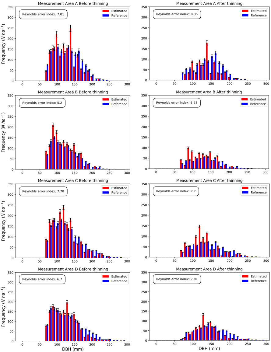
Fig. 5a. Illustration of estimated and reference diameter distributions with uncertainties before and after thinning of measurement areas A–D. Reynold’s error index and visual interpretation indicates that estimated and reference distributions differ only a little. Abbreviation DBH means diameter at breast height.

Fig. 5b. Illustration of estimated and reference diameter distributions with uncertainties before and after thinning of measurement areas E–G. Reynold’s error index and visual interpretation indicates that estimated and reference distributions differ only a little. Abbreviation DBH means diameter at breast height.
4 Discussion
The objectives of this study were to estimate the remaining stem count, diameter distribution, and average basal area of a thinned stand using only data in hpr file after the first thinning operation. In principle, the method had a very clear fundamental setup. The harvested trees from strip roads provide valuable information about the forest before thinning and the quality of operations after thinning. The success of the method relied on the correct detection of the strip road trees, as representative of the entire tree stock before thinning. When identifying the strip road trees, the aim is to collect an optimal sample that is as large as possible, while ensuring it consists only of trees that were within the strip road zone with a very high degree of confidence.
To achieve this, the identification width must be narrower than the actual strip road width that was opened in the forest during the cutting. In Finland, the recommended width of opened strip roads is under 4.6 m on mineral soils and under 5.1 m on peatlands (Tapio Oy 2025). It is also important to note that the width of an opened strip road in the forest is measured differently from the zone width used in this study. The opened strip road in the forest is measured from the remaining strip road edge trees, whereas the zone width in this study was determined based on the felled trees.
In this study, a zone width of 3.2 m was used to identify the strip road trees. This choice was justified because it was based on the width of the harvester. In general, machine model, machine equipment, stand characteristics and harvesting instructions affect also the width parameter. These must be considered stand-wise. Analysis of the harvester data also supported the use of this width (Fig. 3).
Overall, regarding the accuracy of the tree variables before thinning, the harvester data provides accurate information on the cut trees at first thinning, since the measuring accuracy of the harvesters is under frequent monitoring and the harvester volume measurements are used as the basis of payment in Finland (Puutavaranmittauksen neuvottelukunta 2018). Numerically fitting the taper curves (Laasasenaho 1982) is considered the best practice for obtaining stem-wise estimates of DBH and tree height (Suppl. file S1).
The global positioning accuracy of the harvesters has improved considerably due to RTK correction. Together with the parameters of the harvester’s boom position, recorded in the hpr files, the global position of the harvester head can be determined, in practice, to an accuracy level of 0.5 m (Hannrup and Möller 2022; Ylä-Pöntinen et al. 2025). However, the global accuracy is judged to have only a minor effect on the accuracy of these results because it is only relevant in locating the cut hpr trees in the measurement area to obtain reference data on the growing stock before thinning. The accuracy required in this study to identify the strip road trees, based on the boom length and angle, was very high, and some uncertainties remain when using only hpr data.
The geometry of the harvester including the asymmetrical boom attachment caused a bias in the distance distribution of the cut trees. Correcting this bias improved identification of the correct strip road trees. However, the exact position of the harvester head was not available because the rotation angle of the harvester head and the distance between the rotator and the base of the harvester head are currently not recorded in hpr files. Therefore, these details remained unknown when determining the positions of the cut trees. The typical distance between the rotator and the base of the harvester head frame is approximately 15 cm, which can cause inaccuracies in identifying strip road trees. Because of this, at the edge of the sampling zone, either some non-strip road trees may have been included, or some strip road trees excluded from the sample. This distance has been included in the uncertainty analysis via the uncertainty of the GNSS positioning of the harvester data.
The stem counts and basal areas varied substantially between the measurement areas. The estimation of stem counts before thinning was notably accurate for certain measurement areas, with three out of seven measurement areas having the stem counts differ by less than 3% from the reference stem counts. In three other measurement areas, the estimated stem counts differed by approximately 5–14%, which is also considered a good result. However, the basal area was consistently underestimated compared to the reference. In all measurement areas, the relative difference in basal area was systematically lower, regardless of the stem count. The largest relative difference was –10%. This discrepancy can be attributed to an unequal diameter distribution, as visually noted. Strip road trees, as a sample, are also biased towards smaller trees, leading to an underestimation of larger trees in the reference data.
Considering the growing stock after thinning, the results varied. In five out of seven measurement areas, the stem count estimates differed by approximately 7–15% compared to the reference values, while in two measurement areas, the difference was as high as 31%. For basal area after thinning, the same trend was observed as before the operation, the basal area estimates being notably lower, regardless of the stem count. The results of the validation and the uncertainty analysis ( B) indicate that the identification of the strip road trees and the measurement uncertainties are not the main reasons behind the variation of the results. Therefore, there are other factors affecting the results.
In Finland, in a first-thinning stand, the strip roads are opened systematically at 20-m spacings throughout the stand on the decision of the harvester operator. This spacing is maintained almost entirely independently of the trees ahead of the harvester. Only physical obstacles, such as large stones, may force the operator to deviate from the 20-m spacing.
However, it cannot be fully excluded that a harvester operator might favor certain factors in aligning the strip road. When opening a strip road, the harvester operator will consider tree size, quality, and location, natural gaps in the stand, tree density, terrain elevation, obstacles, and other relevant factors (Kärhä et al. 2021). The largest and healthiest trees and trees with the most potential are left to grow. If the strip roads are made through clusters of smaller trees, these will be overemphasized in the diameter distributions. Conversely, if the strip roads go through natural openings, the tree stock volume may be underestimated. The impacts of terrain were observed, with measurement areas with regularly spaced, straight strip roads yielding substantially better results than those where the strip roads curved more and had more crossings. To address this possible source of uncertainty of aligning strip roads through statistically non-representative locations in the measurement area, more information of the initial growing stock would be needed. This topic requires further study.
One important source of uncertainty in the results was the determination of the effective area of the strip road. Because the strip roads cover a relatively small area of the measurement area, small differences in their area can have a major impact on the final estimates. Turns and crossings in the strip road networks affect the area of the strip road. Therefore, strip road samples might benefit from partitioning – for instance, excluding crossings and other irregular parts of the network.
The stem count estimates were more accurate than the basal area estimates. The estimated and reference diameter distributions were very similar (Figs. 5a and 5b), and the Reynold’s error index (1988) being under 10% indicates the same was true for all measurement areas. A visual inspection of the distributions resulted in the same conclusion.
Despite the overall similarity in distributions, some differences remained. The estimated distributions tended to emphasize smaller diameters, which considerably affected the basal area, even though the stem count was similar (Tables 2 and 3). When calculating the stem count by subtracting all the harvested trees from the estimated initial diameter distribution, negative values could occur in some diameter classes if more trees were harvested than initially estimated. In addition, the number of estimated stems in larger-diameter classes (over 200 mm) was generally low. Therefore, replacing the negative diameter distribution values with zero could potentially emphasize the difference in the results of the basal area because the basal area is calculated quadratically from the diameter, increasing the difference at larger diameters. Furthermore, noteworthy peaks in individual diameter classes, such as in measurement areas A and E, may have had a notable effect on the overall results.
One possible explanation for the differences in the diameter distributions was also the number of small trees cut from the strip road versus from the areas between the strip roads. Typically, all the trees are cut from the strip road, even the small ones, whereas some small trees may be left to grow between the strip roads due to the efficiency of the harvesting work. Leaving some small tree clusters benefits game and biodiversity, for example. In addition, using 10-mm classes in diameter distributions is more sensitive to the details than using 20-mm classes, that are also used in the literature (Maltamo et al. 2019).
While the method developed in this study is promising for estimating diameter distributions after first-thinning operations, there are still challenges to address. The underestimation of larger trees and the variability in the results after thinning highlight the need for further refinements to the method. To improve the correspondence between diameter distributions, the application of parametric diameter distributions, such as a Weibull or beta distribution, might smooth out the effects of peaks in individual diameter classes. The positioning accuracy of the harvester head is also expected to improve and become more common in the near future, when harvester manufacturers implement measurement techniques involving the boom and harvester head rotation angle.
In comparison to the Skogforsk method (Hannrup et al. 2015; Bhuiyan et al. 2016), more-accurate input data was used because the boom length including measured boom extension was utilised. The finding of strip road trees having smaller diameters than the rest of the stand’s growing stock were repeated (Bhuiyan et al. 2016). The main difference between this and Skogforsk’s method was the use of foreknown stand data in the latter––such data was not used in this study. Due to this, the results of basal areas after thinning were, on average, slightly biased downward. However, the results from stands with a regular strip road network indicate that the current method can, in such cases, provide quite accurate stem count and basal area estimates of the growing stock after thinning. Notably, the standard deviation in the measurement area -wise basal area was 1.8 m2 ha–1, which is slightly lower than that reported by Hannrup et al. (2015). The largest difference in basal area was 5.2 m2 ha–1 in a measurement area with curvy strip roads with crossings in the middle. On the other hand, when the Skogforsk’s method was tested in Latvia, the estimated diameters of trees after thinning were larger than the manually measured reference diameters (Strubergs et al. 2017). This supports the deduction of the other factors behind the measurement area -wise variation of the results.
Overall, methods based on harvester data have good potential for large-scale use. The method presented in this study could be completely automated with some further study of the details and the establishment of an operational level. Modern harvesters collect a lot of accurate data on a daily basis that is directly applicable in automated methods. Harvester data is, as such, crucial for reporting the quality of thinning operations in forests after thinning. By combining automated methods with harvester data, objective quality assessments can be conducted efficiently at a national level.
Real-time quality management during thinning operations would also become accessible with harvester data. By applying the current approach to parts of a stand’s strip road network, and potentially complementing this with prior forest information, the remaining growing stock can be estimated while the thinning is in progress in the stand. In addition, up-to-date forest information can be obtained from harvester data, improving the accuracy and update interval of open forest information.
5 Conclusions
In this study, a method for estimating tree stem counts and basal areas in stands after the first thinning was introduced. The method is based on the recorded parameters of the harvester boom in harvester hpr files. Currently, Komatsu precision harvesters are recording such data during cutting operations. In the studied method, the strip road trees were identified and used as a sample representative of the initial growing stock, while the remaining growing stock was estimated using diameter distributions. It was found that this method has potential for determining the variables of the remaining growing stock solely from the hpr files in first thinnings. However, further research is needed on the effect of strip road alignment on the selection of strip road trees. As a real-time system, it would also be suitable for the harvester operator’s on-site monitoring of thinning intensity. With further development, this method will be able to provide also large-scale automated reporting and thinning quality management.
Declaration of openness of research materials, data, and code
Restrictions apply to the availability of these data. The data is owned by stakeholders of Metsäteho Oy and is granted for the current purpose.
Author contributions
Conceptualization (all); Methodology (R.T., H.O., K.R. and A.P.); Software (R.T., H.O. and K.R.); Validation (R.T., K.R., and H.O.); Investigation (R.T., H.O. and K.R.); Data Curation (R.T., K.R.); Writing – Original Draft Preparation (R.T.); Writing – Review and Editing, (all); Visualization (R.T., K.R.); Supervision and Project Administration (J.M.); Funding Acquisition (J.M.) All authors have read and agreed to the published version of the manuscript.
Acknowledgments
We thank Metsäteho’s owners and their contractors for their excellent cooperation in collecting the data. Komatsu Forest AB is acknowledged for their assistance with the harvester data. We are grateful to Juha-Antti Sorsa from Metsäteho Oy for helping to prepare the hpr files for our data analyses, and for all the support in several stages of this study. We also thank Timo Melkas from Metsäteho Oy for his support and participation.
Funding of the research
This research has been conducted as a part of Ministry of Agriculture and Forestry program “Nappaa hiilestä kiinni” and as a part of project “Kestävän metsätalouden todentaminen ja menetelmät (KESTOTÄSMÄ)” funded by EU’s Recovery and Resilience Facility (RRF).
References
Bhuiyan N, Möller J J, Hannrup B, Arlinger J (2016) Automatisk gallringsuppföljning. Arealberäkning samt registrering av kranvinkel för identifiering av stickvägsträd och beräkning av gallringskvot. [Automatic follow-up of thinning. Stand area estimation and use of crane angle data to identify strip road trees and calculate thinning quotient]. Arbetsrapport 899, Skogforsk. https://www.skogforsk.se/cd_20190114161523/contentassets/6eda4307138347648171f87e3d9a3885/automatisk-gallringsuppfoljning-arealberakning-samt-registrering-av-kranvinkel-for-identifiering-av-sticktrad-och-berakning-av-gallringskvot-arbetsrapport-899-2016.pdf.
Burström O (2016) Rätt gallringskvalitet med automatisk gallringsuppföljning. [Right quality of thinning with automated follow-up of thinning]. Arbetsrapport 4, Sveriges lantbruksuniversitet, Umeå. https://stud.epsilon.slu.se/9140/.
Cho H-M, Park J-W, Lee J-S, Han S-K (2024) Assessment of the GNSS-RTK for application in precision forest operations. Remote Sens 16, article id 148. https://doi.org/10.3390/rs16010148.
Eriksson M, Lindroos O (2014) Productivity of harvesters and forwarders in CTL operations in northern Sweden based on large follow-up datasets. Int J For Eng 25: 179–200. https://doi.org/10.1080/14942119.2014.974309.
Fassnacht FE, White JC, Wulder MA, Næsset E (2024) Remote sensing in forestry: current challenges, considerations and directions. Forestry 97: 11–37. https://doi.org/10.1093/forestry/cpad024.
Finnish Forest Centre (2025a) Tietotuotekuvaus. [Information product description]. https://www.metsakeskus.fi/sites/default/files/document/tietotuotekuvaus-hila-aineisto.pdf.
Finnish Forest Centre (2025b) Quality of forest resource information. https://www.metsakeskus.fi/en/open-forest-and-nature-information/quality-of-forest-resource-information.
Gollob C, Ritter T, Nothdurft A (2020) Forest inventory with long range and high-speed personal laser scanning (PLS) and simultaneous localization and mapping (SLAM) technology. Remote Sens 12, article id 1509. https://doi.org/10.3390/rs12091509.
Hannrup B, Möller J (2022) Positionering av enskilda träd vid avverkning med skördare. [Positioning of individual trees during harvesting with a harvester.]. Arbetsrapport 1111, Skogforsk. https://wwwmistradigital.cdn.triggerfish.cloud/uploads/2022/03/arbetsrapport-1111-2022.pdf.
Hannrup B, Möller J (2025) Test av förbättrad positionering i skördare. [Testing of improved positioning in a harvester]. Kunskapsartiklar 29, Skogforsk. https://www.skogforsk.se/kunskapsbanken/kunskapsartiklar/2025/test-av-forbattrad-positionering-i-skordare/.
Hannrup B, Bhuiyan N, Möller, JJ (2015) Rikstäckande utvärdering av ett system för automatiserad gallringsuppföljning. [Nationwide evaluation of a system for automated follow-up of thinning]. Arbetsrapport 857, Skogforsk. https://www.skogforsk.se/cd_20190114162402/contentassets/d7aedf5abc1245f78b960b7078f84cae/rikstackande-utvardering-av-ett-system-for-automatiserad-gallringsuppfoljning.pdf.
Hyink DM, Moser JW (1983) A generalized framework for projecting forest yield and stand structure using diameter distributions. For Sci 29: 85–95. https://doi.org/10.1093/forestscience/29.1.85.
Hyyppä M, Turppa T, Hyyti H, Yu X, Handolin H, Kukko A, Hyyppä J, Virtanen J-P (2024) Concepts towards nation-wide individual tree data and virtual forests. ISPRS Int J Geo-Inf 13, article id 424. https://doi.org/10.3390/ijgi13120424.
Kaartinen H, Hyyppä J, Vastaranta M, Kukko A, Jaakkola A, Yu X, Pyörälä J, Liang X, Liu J, Wang Y, Kaijaluoto R, Melkas T, Holopainen M, Hyyppä H (2015) Accuracy of kinematic positioning using global satellite navigation systems under forest canopies. Forests 6: 3218–3236. https://doi.org/10.3390/f6093218.
Kangas A, Maltamo M (2003) Calibrating predicted diameter distribution with additional information in growth and yield predictions. Can J For Res 33: 430–434. https://doi.org/10.1139/x02-121.
Kangas A, Räty M, Korhonen KT, Vauhkonen J, Packalen T (2019) Catering information needs from global to local scales – potential and challenges with national forest inventories. Forests 10, article id 800. https://doi.org/10.3390/f10090800.
Kärhä K, Ovaskainen H, Palander T (2021) Decision-making among harvester operators in tree selection and need for Advanced Harvester Operator Assistant Systems (AHOASs) on thinning sites. Proceedings of the Joint 43rd Annual Meeting of Council on Forest Engineering (COFE) and the 53rd International Symposium on Forest Mechanization (FORMEC); Forest Engineering Family – Growing Forward Together, September 27–30, Corvallis, OR, USA, pp 15–25.
Kilkki P, Maltamo M, Mykkänen R, Päivinen R (1989) Use of the Weibull function in estimating the basal-area diameter distribution. Silva Fenn 23: 311–318. https://doi.org/10.14214/sf.a15550.
Kolmogorov A (1933) Sulla determinazione empirica di una legge di distributione. Giornale dell’ Instituto Italiano degli Attuari 4: 83–91.
Laasasenaho J (1982) Taper curve and volume functions for pine, spruce and birch. Commun Inst For Fenn 108. https://urn.fi/URN:ISBN:951-40-0589-9.
Lee D, Siipilehto J, Hynynen J (2021) Models for diameter distribution and tree height in hybrid aspen plantations in southern Finland. Silva Fenn 55, article id 10612. https://doi.org/10.14214/sf.10612.
Lindroos O, Ringdahl O, La Hera P, Hohnloser P, Hellström T (2015) Estimating the position of the harvester head – a key step towards the precision forestry of the future? Croat J For Eng 36: 147–164.
Lopatin E, Väätäinen K, Kukko A, Kaartinen H, Hyyppä J, Holmström E, Sikanen L, Nuutinen Y, Routa J (2023) Unlocking digitalization in forest operations with viewshed analysis to improve GNSS positioning accuracy. Forests 14, article id 689. https://doi.org/10.3390/f14040689.
Maltamo M, Kangas A (1998) Methods based on k-nearest neighbor regression in the prediction of basal area diameter distribution. Can J For Res 28: 1107–1115. https://doi.org/10.1139/x98-085.
Maltamo M, Hauglin M, Næsset E, Gobakken T (2019). Estimating stand level stem diameter distribution utilizing harvester data and airborne laser scanning. Silva Fenn 53, article id 10075. https://doi.org/10.14214/sf.10075.
Massey F J Jr (1951) The Kolmogorov-Smirnov test for goodness of fit. J Am Stat Assoc 46: 68–78. https://doi.org/10.1080/01621459.1951.10500769.
Melkas T, Riekki K, Sorsa J-A (2020) Automated method for delineating harvested stands based on harvester location data. Remote Sens 12, article id 2754. https://doi.org/10.3390/rs12172754.
Mey R, Temperli C, Stillhard J, Nitzsche J, Thürig E, Bugmann H (2023) Deriving forest stand information from small sample plots: an evaluation of statistical methods. For Ecol Manage 544, article id 121155. https://doi.org/10.1016/j.foreco.2023.121155.
Ministry of Agriculture and Forestry (2021) Suomi kuuluu metsätiedon ja -tietojärjestelmien osalta maailman huippuihin. https://mmm.fi/-/suomi-kuuluu-metsatiedon-ja-tietojarjestelmien-osalta-maailman-huippuihin.
Muhojoki J, Tavi D, Hyyppä E, Lehtomäki M, Faitli T, Kaartinen H, Kukko A, Hakala T, Hyyppä J (2024) Benchmarking under- and above-canopy laser scanning solutions for deriving stem curve and volume in easy and difficult boreal forest conditions. Remote Sens 16, article id 1721. https://doi.org/10.3390/rs16101721.
Ovaskainen H, Riekki K (2022) Computation of strip road networks based on harvester location data. Forests 13, article id 782. https://doi.org/10.3390/f13050782.
Peuhkurinen J, Tokola T, Plevak K, Sirparanta S, Kedrov A, Pyankov S (2018) Predicting tree diameter distributions from airborne laser scanning, SPOT 5 satellite, and field sample data in the Perm Region, Russia. Forests 9, article id 639. https://doi.org/10.3390/f9100639.
Puutavaranmittauksen neuvottelukunta (2018) Hakkuukoneen mittaustarkkuuden ylläpito. [Maintenance of harvester measurement accuracy]. https://urn.fi/URN:NBN:fi-fe2018092836899.
QGIS.org (2025) QGIS Geographic Information System. http://www.qgis.org.
Räsänen T, Melkas T, Riekki K, Sorsa J-A, Poikela A, Hämäläinen J (2019) Hakkuukoneet metsätiedon tuottajina. [Harvesters as producers of forest data]. Metsätieteen aikakauskirja, article id 10250. https://doi.org/10.14214/ma.10250.
Reynolds M, Burk T, Huang W (1988) Goodness-of-Fit tests and model selection procedures for diameter distribution models. For Sci 34: 373–399. https://doi.org/10.1093/forestscience/34.2.373.
Skogforsk (2025) StanForD 2010. Standard for forest machine data and communication. http://www.skogforsk.se/english/projects/stanford/.
Stendahl J, Dahlin B (2002) Possibilities for harvester-based forest inventory in thinnings. Scand J For Res 17: 548–555. https://doi.org/10.1080/02827580260417206.
Strubergs A, Zimelis A, Kaleja S, Ivanovs J, Sisenis L, Lazdiņš A (2017) Using cut-to-length (CTL) Harvester production data in forest inventories. Croat J For Eng 45: 277–292. https://doi.org/10.5552/crojfe.2024.2319.
Tapio Oy (2025) Metsänhoidon suositukset. [Best Practice Guidelines for Sustainable Forest Management]. https://tapio.fi/projektit/metsanhoidon-suositukset.
Taylor J (1982) An introduction to error analysis. University Science Books.
Vähä-Konka V, Korhonen L, Kärhä K, Maltamo M (2025) Estimating timber assortment reduction and sawlog proportions with the application of harvester measurements and open big geodata. Trees For People 20, article id100811. https://doi.org/10.1016/j.tfp.2025.100811.
Ylä-Pöntinen J, Ovaskainen H, Tarvainen R, Riekki K, Melkas T, Kärhä K, Malinen J (2025) Hakkuukoneen paikannuksen tarkkuus ja ajourapuuston hyödyntäminen lähtöpuuston määrittämisessä. [Positioning accuracy of a harvester and utilization of strip road trees to determine the initial stand attributes of harvesting site]. Metsätehon tuloskalvosarja 6/2025. https://www.metsateho.fi/hakkuukoneen-paikannuksen-tarkkuus-ja-ajourapuuston-hyodyntaminen-lahtopuuston-maarittamisessa/.
Total of 43 references.
