Michał Zasada 
Evaluation of the double normal distribution for tree diameter distribution modeling
Zasada M. (2013). Evaluation of the double normal distribution for tree diameter distribution modeling. Silva Fennica vol. 47 no. 2 article id 956. https://doi.org/10.14214/sf.956
Abstract
The double normal distribution consists of two normal distributions truncated at their means and then combined in such a way, that points of truncation now become the overall distribution mode. So far, parameters of the double normal distribution have been estimated exclusively using the method of moments. This study evaluates the maximum likelihood method for the estimation of the double normal distribution parameters in Scots pine stands in Poland, and compares it to the results of the method of moments and the two-parameter Weibull distribution fitted using the maximum likelihood method and the method of moments. Presented results show that it is not recommended to use the maximum likelihood method of parameter fitting with Nelder-Mead and quasi-Newton optimization algorithms for the double normal distribution for small samples. However, it can be used for large samples, giving the fit comparable to the two-parameter Weibull distribution and providing parameters having sound practical and biological meaning. In the case of smaller samples for the double normal distribution it is recommended to apply the maximum likelihood method with the alternative simulated annealing optimization algorithm, use the method of moments or substitute the described distribution with more the flexible and robust Weibull distribution. For the smaller samples, the method of moments was superior to the maximum likelihood method.
Keywords
diameter distribution;
simulated annealing;
goodness-of-fit;
Weibull distribution;
maximum likelihood method;
method of moments
-
Zasada,
Warsaw University of Life Sciences, Faculty of Forestry, Laboratory of Dendrometry and Forest Productivity, Nowoursynowska 159, 02-776 Warsaw, Poland
E-mail
michal.zasada@wl.sggw.pl
Received 12 November 2012 Accepted 18 March 2013 Published 1 July 2013
Views 167205
Available at https://doi.org/10.14214/sf.956 | Download PDF

1 Introduction
For more than a hundred years foresters have written about how to describe stand diameter distributions using theoretical models, especially as a part of building volume and yield tables and growth models. Much research has been done on the utilization of various theoretical functions for diameter distribution modeling, such as Gram-Charlier series (Cajanus 1914), geometrical series, proposed by de Liocourt, an exponential form of the de Liocourt model (Meyer and Stevenson 1943; Meyer 1952; Leak 1964), Pearson distributions (Schnur 1934), Pearl-Reed growth curves (Osborne and Schumacher 1935; Nelson 1964), gamma distribution (Nelson 1935), lognormal distribution (Bliss and Reinker 1964), beta distribution (Clutter and Bennett 1965; McGee and Della-Bianca 1967; Lenhard and Clutter 1971), Weibull distribution (Bailey and Dell 1973) , logit-logistic distribution (Wang and Rennols 2005), SB Johnson distribution (Hafley and Shreuder 1977; Siekierski 1992) and Birnbaum–Saunders distribution (Podlaski 2008). Recently, there were also a few results published on the use of the mixture distribution for the modeling of tree diameter distribution in stands with more complex structure (Zhang et al. 2001; Liu et al. 2002; Zasada and Cieszewski 2005; Podlaski 2010; Podlaski 2011). Nowadays, because of its properties and advantages, one of the most frequently used has been the Weibull distribution, especially in its 3-parameter and, if necessary, truncated version (see Merganič and Sterba 2006). However, Maltamo et al. (1995) found 2-parameter Weibull to perform better than the 3-parameter one. Despite many successful applications of various functions, there is still a lot of research being done to find alternative functions and parameter estimation methods that could provide a better fit of models to the data or give more practical interpretations of their parameters.
One example of such an effort is the double normal distribution. Bruchwald (1988) used this newly developed distribution for tree diameter description in a growth model for even-aged stands of Scots pine (Pinus sylvestris L.). Siekierski (1991) provided the description of various methods of parameter estimation for the double normal distribution. The double normal distribution was later used for tree diameter modeling of other species such as true fir (Abies alba Mill.) (Zasada 1995), beech (Fagus sylvatica) (Rymer-Dudzińska and Dudzińska 2001), and birch (Betula) (Zasada 2000). The described distribution was also used as an element of growth models for Scots pine (Bruchwald 1986; Bruchwald 1991), Norway spruce (Picea abies L.) (Bruchwald et al. 1999), true fir (Zasada 1999), and oak (Quercus) (Bruchwald et al. 1996), developed in Poland.
So far, parameters of the double normal distribution have been estimated exclusively using the method of moments (Siekierski 1991), which in some cases reveals limitations. The aim of this study was to:
- evaluate the maximum likelihood method (MLM) for the estimation of the double normal distribution parameters in Scots pine stands,
- compare the maximum likelihood estimates to different variants of the method of moments (MOM) for the double normal distribution Siekierski (1991) and for the Weibull distribution,
- compare the double normal distribution to the two-parameter Weibull distribution, which has been the most widely used for tree diameter distribution modeling in forestry, and
- evaluate and compare the performance of the double normal and two-parameter Weibull distributions in estimation of parameters in cases where one has to deal with small samples.
2 Material and methods
The double normal distribution consists of two normal distributions N(m, s1) and N(m, s2) truncated at their means “m” and then combined in such a way, that points of truncation now become the new distribution mode “m0“ (Fig. 1). The probability density function of this distribution, published by Siekierski (1991), has the following form:
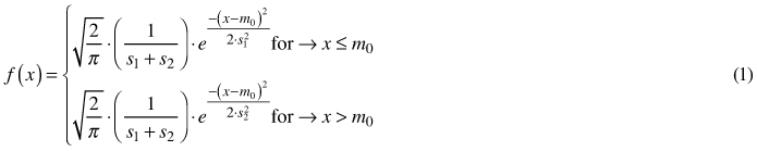
where x is a random variable, m0 is the mode of the distribution, s1 is the standard deviation of the left half of the distribution, and s2 is the standard deviation of the right half of the distribution.
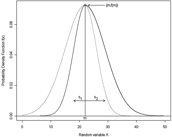
Fig. 1. A sample graph of the double normal distribution with m = 22, s1 = 4 and s2 = 7. Notation: m – the mean of the compound distributions that becomes an overall distribution mode, s1 – the standard deviation of the first compound distribution, which makes a left half of the overall distribution, s2 – the standard deviation of the second compound distribution, which makes a right half of the overall distribution; solid lines show the resulting double normal distribution.
The cumulative distribution function (cdf) of the double normal distribution is not available in a closed form because Eq. 1 is not analytically integrable. However, values of the cdf can be determined numerically, as in the normal distribution, using the value of the “error function” (erf), and the following equations:
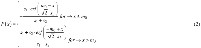
where  = F(x = m0).
In the study the diameter distribution data of 20 well-stocked, pure, even-aged Scots pine (Pinus sylvestris L.) stands was provided by the Department of Dendrometry and Forest Productivity at the Faculty of Forestry in Warsaw, Poland. The sample plots were located on typical pine sites (coniferous forest habitat) in Bory Tucholskie in north-central Poland. Areas of plots were set such that they comprised a few hundred trees. The diameters at breast height (dbh) of all trees were measured on the sample plots with an accuracy of 1 mm. Each plot was characterized by the following attributes: i) average total age, determined by counting rings on stumps of felled trees and sample cores; ii) average height, defined using the Lorey formula (basal area weighted average height); iii) site index, defined as the average height of the 100 thickest trees per hectare at base age 100 years, and calculated using the site index model for Scots pine in Poland (Bruchwald et al. 2000; Cieszewski and Zasada 2002); iv) basal area (BA), mean diameter (MD) and quadratic mean diameter (QMD). Table 1 summarizes the univariate statistics for the data used in the analysis.
| Table 1. Summary statistics of the 20 sample plots used in the study. | ||||||||
| Area | Age | N | QMD | MD | HL | BA | SI | |
| [ha] | [years] | [trees] | [cm] | [cm] | [m] | [m2 ha–1] | [m] | |
| Minimum | 0.049 | 26 | 258 | 6.2 | 5.9 | 7.70 | 22.40 | 16.90 |
| Maximum | 0.810 | 123 | 500 | 28.7 | 28.3 | 23.20 | 31.20 | 27.20 |
| Average | 0.297 | 58 | 378 | 15.5 | 15.0 | 14.34 | 27.18 | 22.03 |
| Std dev. | 0.235 | 25 | 67 | 6.0 | 5.9 | 3.70 | 2.55 | 3.53 |
| Notation: Area – size of the sample plot; Age – average stand age; N – number of trees per plot; QMD – quadratic mean diameter of the stand (calculated from BA and N); MD – mean diameter (arithmetic mean of breast height diameter); HL – average stand height calculated using the Lorey formula (basal area weighted average height); BA – basal area per hectare; SI – base-age 100 site index (Bruchwald et al. 2000; Cieszewski and Zasada 2002). | ||||||||
As it was already mentioned, so far, parameters of the double normal distribution have been estimated exclusively using the method of moments (Siekierski 1991). Moments are numerical characteristics of a probability distributions or population, and can be calculated as raw (simple, ordinary, crude) moments, calculated about the origin (zero), and central ones, calculated about the arithmetic mean (or other value). Since we usually don’t have information on an entire population, we use a sample drawn from the population to estimate population moments.
The kth ordinary moment of the probability distribution is defined as:
![]()
The kth simple sample moment mk is defined as:

The kth central moment of the probability distribution is defined as:
![]()
The kth central sample moment mk is defined as:

where k is an integer number ≥1, E(●) is an expected value, X is a random variable, F(x) is a probability density function, xi are elements sampled from the population, m is the arithmetic mean, and n is the sample size (Wooldridge 2001; Vrbik 2005; Encyclopedia 2012).
Note, that the first raw moment is the mean, the second central moment equals variance, and third moment corresponds to the distribution skewness. Sample moments are function of means of various powers of xi derived from a sample, thus they are random variables. Theoretical moments (moments of the probability distribution) are related to the population, so they are non-random functions of the variable distribution and they are calculated from its parameters. Each kth central moment can be expressed as a function of raw moments of the order ≤ k.
The method of moments is a technique for obtaining estimators of the distribution parameters that is based on matching the sample moments with the corresponding distribution moments and solving for a system of k equations with k unknowns. The method of moments in some cases reveals limitations. For example, the estimates given by the method of moments can be outside of the parameter space, especially for small samples. Moreover, estimates by the method of moments don’t take into account all information included in the sample. The MOM produces in most cases unbiased estimators, however they may not be the most efficient ones.
An alternative to the method of moments is the maximum likelihood method, first described by Fisher in 1922. It is a general method of parameter estimation for the population attribute distribution that maximizes the likelihood function of the sample (Fisher 1922). The likelihood function L of the n-element sample x1, x2, ..., xn, is the joint probability function p(x1, x2, ..., xn), where x1, x2, ..., xn are the independent instances of a discrete random sample or a joint probability density function f(x1, x2, ..., xn), when x1, x2, ..., xn are detailed values of the continuous random variable. Likelihood function L can be written in the following parametrical form:

where ψ is a complete set of the density function parameters to be found. This function determines the chance of an occurrence that ψ is a „true” set of unknown parameters in such a situation, when the exact series of results x1, x2, …, xn was obtained in the sample. The best estimation of the parameters occurs for such a value of ψ that the likelihood function reaches its maximum. Such parameters are called maximum likelihood estimates or MLE. If the likelihood function can be differentiated, such conditions are fulfilled if:
 , assuming that
In practice, the maximum likelihood method maximizes the log of the likelihood function or, equivalently, minimizes the negative log of the likelihood function, for which the extremes are the same as for the original likelihood function L:

assuming that 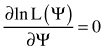
The set of parameters ψ is usually estimated by minimizing the negative log-likelihood using some iterative method available in most statistical packages and languages.
In the presented study the distribution parameters for the double normal and for the Weibull distributions were estimated using the maximum likelihood method implemented using an optimization based on Nelder-Mead and quasi-Newton algorithms. The alternative simulated annealing optimization algorithm has also been applied for small samples. The initial values for the double normal distribution were calculated based on the analysis of the complete data compared to the mean m0, s1 and s2 parameter values estimated for each sample plot from repeated samples. The starting value of m0 was set to 90% of the sample mean, s1 to 70% of the standard deviation of the sample and s2 to the standard deviation of the sample increased by 30%. The initial parameters of the Weibull distribution were calculated based on the mean and standard deviation of the sample using the weibullpar function from the mixdist package of the R software (Macdonald 2010).
Parameters of the double normal distribution were also fit by means of the method of moments (Siekierski 1991). The following variants of the MOM were used: MOM3, using first three moments of the sample (Eqs. 9, 10 and 11), and MOM2, using two first moments of the sample (Eqs. 9 and 10) and the distribution mode estimated using the approximate formula: m0 = m – 4.8 · (m – me), where me equals to the median. First three moments were calculated according to the following equations (Siekierski 1991):


where mk is a kth moment, m corresponds to the arithmetic mean of the truncated normal distributions (m0 of the joined double normal distribution), and sj equals to the standard deviation of the left and right tail of the double normal distribution.
Also, for comparison, parameters of the two-parameter Weibull distribution were fit by means of the method of moments using two first moments of the sample (MOM2W), as described e.g. by Al-Fawzan (2000), Gove 2003 or Lei (2008). The kth moment of the Weibull distribution is expressed by the following equation:

where b – scale parameter, c – shape parameter of the distribution, Γ – gamma function. Thus, the first and the second moments of the distribution (m1 and m2) were calculated as follows:

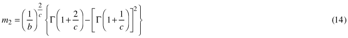
By dividing m2 (Eq. 14) by the square of m1 (Eq. 13), and taking the square root of this ratio, we obtain the coefficient of variation (CV), which relies exclusively on the c parameter:
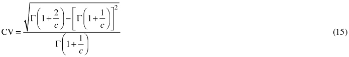
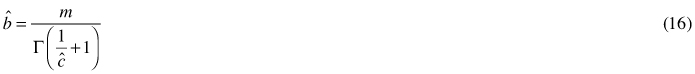
Eq. 15 was solved using the root-finding bisection procedure (Forsythe et al. 1977) to obtain the estimate of ![]() . The scale parameter b was finally obtained using the following equation (Shifley and Lentz 1985; Gorgoso et al. 2007):
. The scale parameter b was finally obtained using the following equation (Shifley and Lentz 1985; Gorgoso et al. 2007):
Parameters were also calculated using the simplified method of moments described by García (1981).
In all cases the goodness-of-fit was tested using the Kolmogorov-Smirnov test (Dn statistic).
Sample plots used in the study consisted of a few hundred trees. This fact dramatically limits practical conclusions obtained from analyses, since in forest inventory foresters usually deal with much smaller numbers of measurements per plot. To address this problem, analyses were also performed using random subsets of 10 and 50 measurements taken 100 times from each sample plot. Samples drawn for each plot were characterized using the number of failed estimations at 0.05 significance level and the average Kolmogorov-Smirnov Dn statistic.
All analyses were performed using programs written in the R language (Ihaka and Gentleman 1996, see an example code for the maximum likelihood method for fitting parameters of the double normal distribution and the method of moments for the parameters of the Weibull distribution in the Appendix).
3 Results
When analyzing all trees from sample plots, the hypothesis that empirical distributions match distributions with fitted parameters could not be rejected in any analyzed case. The maximum likelihood method for the double normal distribution was superior to the both variants of the method of moments in 9 out of 20 analyzed plots, however the differences were very small, sometimes almost negligible. The method of moments for the Weibull distribution was superior to the maximum likelihood method in 14 out of 20 analyzed plots, however, as in the case of the double normal distribution, the differences were very small, sometimes almost negligible. Results obtained from the simplified method of moments by García (1981) were practically identical to the classical method (Eqs. 13–16), so they were not reported nor analyzed separately. The double normal distribution slightly overtook the Weibull distribution in 9 cases out of 20 plots (regardless the fitting method). The average values of the Dn statistic of the Kolmogorov-Smirnov test were slightly higher for the double normal distribution than for the Weibull distribution, which indicates a slightly poorer overall performance (overall fit) of this distribution. The best overall performance revealed the Weibull distribution with parameters fit using the method of moments. Detailed values of the Dn statistic for various methods of parameter fitting for the double normal distribution and the Weibull distribution are presented in Table 2. The typical graphs of the fitted distributions are presented in Figs. 2 and 3. In both cases the double normal distribution is more positively skewed and has higher maximum frequency for the modal value than the Weibull distribution. The double normal distribution is inferior to the Weibull distribution in cases when the distribution becomes symmetrical or negatively skewed.
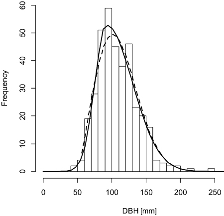
Fig. 2. A sample graph of the double normal distribution (solid line) outperforming the Weibull distribution (dashed line) for the plot BT119 (histogram).
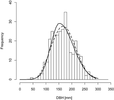
Fig. 3. A sample graph of the Weibull distribution (dashed line) outperforming the double normal distribution (solid line) for the plot BT130 (histogram).
| Table 2. Detailed values of the Dn statistics for various distributions and methods of fitting. MLE denotes the maximum likelihood method, MOM3 – method of moments based on first three moments of the sample, MOM2 – method of moments based on first two moments of the sample and the distribution mode estimated using the approximate formula: mode = mean – 4.8 · (mean – median), MOM2W – method of moments based on first two moments of the sample. Lower value of the Dn statistics denote better fit. The best fit is marked with bold numbers. | |||||
| Double normal | Weibull | ||||
| Plot | MLE | MOM3 a) | MOM2 a) | MLE | MOM2W |
| BT112 | 0.0356 | 0.0327 | 0.0327 | 0.0324 | 0.0317 |
| BT113 | 0.0347 | 0.0285 | 0.0285 | 0.0294 | 0.0282 |
| BT114 | 0.0452 | 0.0542 | 0.0542 | 0.0568 | 0.0613 |
| BT115 | 0.0391 | 0.0490 | 0.0490 | 0.0373 | 0.0412 |
| BT116 | 0.0385 | 0.0413 | 0.0413 | 0.0422 | 0.0428 |
| BT117 | 0.0344 | 0.0355 | 0.0355 | 0.0380 | 0.0378 |
| BT118 | 0.0453 | 0.0294 | 0.0294 | 0.0255 | 0.0249 |
| BT119 | 0.0244 | 0.0399 | 0.0399 | 0.0384 | 0.0343 |
| BT120 | 0.0572 | 0.0396 | 0.0396 | 0.0345 | 0.0321 |
| BT121 | 0.0277 | 0.0441 | 0.0441 | 0.0379 | 0.0375 |
| BT122 | 0.0317 | 0.0355 | 0.0355 | 0.0310 | 0.0310 |
| BT123 | 0.0315 | 0.0310 | 0.0310 | 0.0212 | 0.0211 |
| BT124 | 0.0253 | 0.0197 | 0.0197 | 0.0275 | 0.0271 |
| BT125 | 0.0221 | 0.0261 | 0.0261 | 0.0474 | 0.0406 |
| BT126 | 0.0394 | 0.0476 | 0.0476 | 0.0552 | 0.0462 |
| BT127 | 0.0322 | 0.0283 | 0.0283 | 0.0264 | 0.0302 |
| BT128 | 0.0340 | 0.0323 | 0.0323 | 0.0289 | 0.0298 |
| BT129 | 0.0391 | 0.0349 | 0.0349 | 0.0397 | 0.0386 |
| BT130 | 0.0361 | 0.0354 | 0.0354 | 0.0273 | 0.0277 |
| BT131 | 0.0499 | 0.0390 | 0.0390 | 0.0315 | 0.0270 |
| Avg. | 0.0362 | 0.0362 | 0.0362 | 0.0354 | 0.0346 |
| a) Values of the Dn statistics for MOM2 and MOM3 are not identical, but the differences exist below the resolution of the presentation of results. | |||||
As the sample size decreases, the average goodness-of-fit decreases (Tables 3 and 4). For medium-size samples of 50 trees the best results were obtained for the Weibull distribution with parameters fitted using the maximum likelihood method. The Weibull distribution was superior to the double normal distribution on average in 16 cases out of 20. The maximum likelihood method gave on average a better fit than the method of moments, however it occasionally failed to converge. For the double normal distribution the method of moments gave on average a better fit than the maximum likelihood method, and the MOM3 variant (parameters fitted using first three moments of the sample) was better than the MOM2 one (method based on two first moments of the sample and the distribution mode estimated using the approximate formula), but comparison of detailed values for particular plots is not clear. The detailed values of the Dn statistic and the number of cases when the hypothesis of matching empirical and theoretical distributions was rejected are presented in Table 3.
| Table 3. Detailed values of the Dn statistics and number of cases when the hypothesis about matching the empirical and theoretical distributions was rejected for various distributions and methods of fitting for 100 samples of 50 trees. For explanations of the abbreviations see Table 2. MLE(S) – the maximum likelihood method with simulated annealing optimization algorithm. The best fit without MLE(S) method is marked with bold numbers, and with the MLE(S) – with underlined numbers. | ||||||||||||
| Plot | Double normal | Weibull | ||||||||||
| MLE | 0.05 | MLE(S) | 0.05 | MOM3 | 0.05 | MOM2 | 0.05 | MLE | 0.05 | MOM2W | 0.05 | |
| BT112 | 0.0973 | 7 | 0.0753 | 0 | 0.0811 | 0 | 0.0890 | 0 | 0.0674 | 0 | 0.0660 | 0 |
| BT113 | 0.0967 | 8 | 0.0715 | 0 | 0.0698 | 0 | 0.0756 | 0 | 0.0670 | 0 | 0.0652 | 0 |
| BT114 | 0.1054 | 7 | 0.0845 | 4 | 0.1533 | 0 | 0.0859 | 0 | 0.0855 | 1 | 0.0894 | 0 |
| BT115 | 0.0906 | 2 | 0.0798 | 2 | 0.0985 | 0 | 0.0793 | 0 | 0.0802 | 0 | 0.0771 | 0 |
| BT116 | 0.1329 | 12 | 0.0752 | 0 | 0.0733 | 0 | 0.0789 | 0 | 0.0670 | 0 | 0.0729 | 0 |
| BT117 | 0.1352 | 14 | 0.0773 | 0 | 0.0867 | 0 | 0.0847 | 0 | 0.0757 | 0 | 0.0752 | 0 |
| BT118 | 0.1168 | 9 | 0.0773 | 1 | 0.0691 | 0 | 0.0741 | 0 | 0.0697 | 0 | 0.0711 | 0 |
| BT119 | 0.1078 | 6 | 0.0776 | 0 | 0.1251 | 0 | 0.0910 | 0 | 0.0789 | 0 | 0.0781 | 0 |
| BT120 | 0.1563 | 18 | 0.0799 | 0 | 0.0877 | 0 | 0.0900 | 0 | 0.0758 | 0 | 0.0794 | 0 |
| BT121 | 0.1193 | 12 | 0.0720 | 0 | 0.0753 | 0 | 0.0791 | 0 | 0.0687 | 1 | 0.0706 | 0 |
| BT122 | 0.1738 | 20 | 0.0735 | 0 | 0.0785 | 0 | 0.0776 | 0 | 0.0660 | 0 | 0.0690 | 0 |
| BT123 | 0.1794 | 22 | 0.0726 | 0 | 0.0890 | 0 | 0.0753 | 0 | 0.0627 | 0 | 0.0608 | 0 |
| BT124 | 0.1350 | 15 | 0.0718 | 1 | 0.0978 | 0 | 0.0693 | 0 | 0.0703 | 2 | 0.0683 | 0 |
| BT125 | 0.0756 | 2 | 0.0857 | 1 | 0.0743 | 0 | 0.0726 | 0 | 0.0768 | 1 | 0.0747 | 0 |
| BT126 | 0.0825 | 1 | 0.0750 | 1 | 0.0896 | 0 | 0.0819 | 0 | 0.0889 | 2 | 0.0914 | 0 |
| BT127 | 0.0838 | 2 | 0.0709 | 0 | 0.0783 | 0 | 0.0829 | 0 | 0.0723 | 0 | 0.0700 | 0 |
| BT128 | 0.1013 | 5 | 0.0740 | 0 | 0.0778 | 0 | 0.0830 | 0 | 0.0684 | 0 | 0.0748 | 0 |
| BT129 | 0.0971 | 5 | 0.0735 | 0 | 0.0855 | 0 | 0.0886 | 0 | 0.0769 | 1 | 0.0683 | 0 |
| BT130 | 0.0946 | 5 | 0.0767 | 0 | 0.0697 | 0 | 0.0774 | 0 | 0.0716 | 0 | 0.0743 | 0 |
| BT131 | 0.1133 | 8 | 0.0780 | 0 | 0.0912 | 0 | 0.0829 | 0 | 0.0727 | 0 | 0.0769 | 0 |
| Avg. | 0.1147 | 0.0761 | 0.0876 | 0.0809 | 0.0731 | 0.0737 | ||||||
A further decrease in performance was observed for small samples of 10 trees (Table 4). In this case the worst appeared to be the double normal distribution, especially its variant with parameters fitted using the maximum likelihood method, which not only had the average value of the Dn statistic indicating lack of fit for 43% of samples at 0.05 significance level, but also in many cases did not reach the convergence of fitting. The Weibull distribution was able to provide a good fit to the data almost every time for each sample, and was followed by the method of moments for the double normal distribution, which did not provide good fitting only in a few cases. The average value of the Dn statistic for the double normal distribution and maximum likelihood method was more than two times higher than for the method of moments and for the Weibull function.
| Table 4. Detailed values of the Dn statistics and number of cases when the hypothesis about matching the empirical and theoretical distributions was rejected for various distributions and methods of fitting for 100 samples of 10 trees. For explanations of the abbreviations see Table 2. The best fit is marked with bold numbers. | ||||||||||||
| Plot | Double normal | Weibull | ||||||||||
| MLE | 0.05 | MLE(S) | 0.05 | MOM3 | 0.05 | MOM2 | 0.05 | MLE | 0.05 | MOM2W | 0.05 | |
| BT112 | 0.3519 | 45 | 0.1857 | 6 | 0.1678 | 1 | 0.1755 | 1 | 0.1472 | 0 | 0.1391 | 0 |
| BT113 | 0.3210 | 37 | 0.2050 | 12 | 0.1555 | 2 | 0.1562 | 1 | 0.1387 | 0 | 0.1379 | 1 |
| BT114 | 0.4111 | 53 | 0.2461 | 15 | 0.2076 | 4 | 0.1735 | 0 | 0.1577 | 0 | 0.1590 | 1 |
| BT115 | 0.3605 | 39 | 0.1953 | 4 | 0.1823 | 2 | 0.1675 | 0 | 0.1482 | 0 | 0.1529 | 0 |
| BT116 | 0.3478 | 40 | 0.1891 | 3 | 0.1745 | 2 | 0.1698 | 1 | 0.1394 | 0 | 0.1408 | 0 |
| BT117 | 0.3947 | 50 | 0.2154 | 9 | 0.1894 | 4 | 0.1786 | 3 | 0.1528 | 2 | 0.1466 | 0 |
| BT118 | 0.3348 | 38 | 0.1868 | 3 | 0.1530 | 2 | 0.1556 | 1 | 0.1478 | 0 | 0.1407 | 2 |
| BT119 | 0.3604 | 44 | 0.2275 | 7 | 0.1867 | 3 | 0.1722 | 3 | 0.1536 | 0 | 0.1499 | 1 |
| BT120 | 0.4047 | 50 | 0.2154 | 7 | 0.1698 | 3 | 0.1708 | 2 | 0.1510 | 1 | 0.1466 | 0 |
| BT121 | 0.3522 | 42 | 0.2059 | 3 | 0.1690 | 1 | 0.1724 | 1 | 0.1290 | 0 | 0.1358 | 0 |
| BT122 | 0.4264 | 56 | 0.1979 | 9 | 0.1782 | 2 | 0.1688 | 0 | 0.1473 | 0 | 0.1362 | 1 |
| BT123 | 0.3514 | 39 | 0.2031 | 9 | 0.1742 | 1 | 0.1567 | 1 | 0.1419 | 0 | 0.1382 | 1 |
| BT124 | 0.3946 | 50 | 0.1671 | 2 | 0.1657 | 1 | 0.1576 | 0 | 0.1325 | 0 | 0.1350 | 0 |
| BT125 | 0.3530 | 40 | 0.1739 | 4 | 0.1642 | 2 | 0.1677 | 2 | 0.1611 | 0 | 0.1485 | 1 |
| BT126 | 0.3227 | 36 | 0.1791 | 3 | 0.1806 | 3 | 0.1619 | 0 | 0.1636 | 0 | 0.1536 | 0 |
| BT127 | 0.3840 | 49 | 0.1700 | 0 | 0.1451 | 0 | 0.1478 | 0 | 0.1565 | 0 | 0.1488 | 0 |
| BT128 | 0.3413 | 38 | 0.1839 | 1 | 0.1616 | 5 | 0.1607 | 3 | 0.1626 | 1 | 0.1402 | 0 |
| BT129 | 0.3259 | 35 | 0.1923 | 6 | 0.1644 | 2 | 0.1725 | 1 | 0.1648 | 0 | 0.1388 | 0 |
| BT130 | 0.3322 | 38 | 0.1894 | 7 | 0.1716 | 2 | 0.1812 | 1 | 0.1668 | 1 | 0.1447 | 2 |
| BT131 | 0.3324 | 36 | 0.1849 | 4 | 0.1669 | 1 | 0.1636 | 1 | 0.1586 | 2 | 0.1524 | 2 |
| Avg. | 0.3602 | 0.1958 | 0.1714 | 0.1665 | 0.1511 | 0.1443 | ||||||
4 Discussion and conclusions
Maximum likelihood estimates can be heavily biased for small samples. Also, the parameter optimality property may not apply for small samples. In the presented study this was proven mostly for the double normal distribution, especially fitted to the data from 10-tree samples. Also, the maximum likelihood method appeared to be sensitive to the choice of starting values, again – mostly in the case of the double normal distribution. Even using starting values initially approximated by the method of moments did not assure a good fit to the data.
For big samples, the performance (measured by the Dn Kolmogorov statistic) of the analyzed distributions was comparable. The Weibull distribution was superior to the double normal one. The maximum likelihood method for the Weibull distribution appeared to be superior to the method of moments, which confirms results obtained by Shiver (1988). At the same time the MLM failed to converge in a few cases. After replacing the default Nelder-Mead (NM) optimization method with the simulated annealing (SANN) approach (chosen after checking also other possible fitting methods such as quasi-Newton (qN), gradient and box constraints) the overall Dn statistics did not improve, but the algorithm achieved the convergence in most cases. The maximum likelihood method of parameter estimation applied to the double normal distribution always gave the poorest performance. This was a surprising outcome taking into account results obtained from the Weibull distribution. After detailed check of the parameters it was noticed that worse overall fit statistics are caused mainly by the unrealistic parameter values which denote the failure of the fitting algorithm. Changing initial parameters did not improve fitting statistics, but optimization algorithm replaced with the SANN method gave desirable results: average fit statistics as well as the number of cases with unrealistic values decreased. The maximum likelihood method for the double normal distribution gave in this case better results than the method of moments, but worse than both analyzed methods of parameter calculations for the Weibull distribution. It outperformed the Weibull distribution only in the case of two plots (see values in the MLE(S) column in Table 3).
The trends of decreasing goodness-of-fit and increasing number of failed fits continued for smaller samples and finally practically disqualified the maximum likelihood method of parameter estimation for the double normal distribution. It was not possible to obtain a fit of the distribution to the data for most of the analyzed plots. Much more robust appeared to be the method of moments, which was able to provide satisfactory fits for medium-size, and also in many cases for the small-size samples.
In the case of the samples consisting of 10 element, poor performance of the maximum likelihood method applied to the double normal distribution can be caused by such factors as: small sample size, giving not enough information to fit the correct parameters, wrong choice of the starting parameters, failure in finding reasonable values of parameters and the optimization method applied in the MLM. In order to find the source of the problems, the extensive analysis was done, following the scheme described for 50-element samples.
First, the detailed values of parameters were checked. In many cases their values were clearly wrong (e.g. negative means and standard deviations), which denotes problems with the fitting process. In order to check whether the problem exists because of the inappropriate starting values of parameters, they were replaced with the values i) calculated using the method of moments from the sample and ii) calculated using the method of moments from the complete plot data. None of the approaches significantly changed the results: the average Dn statistics, as well as the number of failed fits, were the same.
Then, the influence of the optimization algorithm on the results was tested. The default NM and qN methods were replaced with the simulated annealing (SANN) method. The application of this algorithm lowered the average Dn statistics by about a half, but still placed the double normal distribution with parameters fitted using MLM behind the method of moments and the Weibull distribution. The number of failed fits (unrealistic parameters, mostly negative standard deviations of the left part of the distribution) significantly decreased (see values in the MLE(S) column in Table 4).
Clearly, one of the major factors influencing the results obtained for the double normal distribution analysis using small samples is the choice of the optimization method used in the MLM. Simulated annealing algorithm was much more resistant to the bad choice of starting values caused by a small sample size than the NM and qN. However, at the same time, the SANN approach appeared to be more time consuming than other methods. Another factor influencing the fitting process is the choice of the initial parameters. This is especially complicated process when small samples, providing very variable values, are taken into account. One of the solutions of this issue is the use of the method described by Mehtätalo et al. (2011).
Presented results discourage from using the maximum likelihood method of parameter fitting for the double normal distribution for small samples using NM and qN optimization methods. It can be used for larger samples, giving the fit comparable to the Weibull distribution, and providing, similarly to the Weibull distribution, parameters having sound practical and biological meaning. In case of smaller samples for the double normal distribution it is recommended to apply SANN optimization method, use the method of moments or substitute the described distribution with the more flexible and robust Weibull distribution.
The results presented in this study confirm that the most efficient procedure for fitting the parameters of the diameter distribution is to use the maximum likelihood method with initial values of parameters calculated using the method of moments from the sample data. This approach has proved to be useful for both analyzed distributions. It was also concluded that it is very important to choose a robust optimization algorithm of the applied MLM. This is especially important for small and medium samples, where SANN was much slower, but at the same time much more reliable than the NM and qN methods.
References
Al-Fawzan M.A. (2000). Methods for estimating the parameters of the Weibull distribution. King Abdulaziz City for Science and Technology, Saudi Arabia.
Bailey R.L., Dell T.R. (1973). Qualifying diameter distributions with the Weibull function. Forest Science 19: 97–104.
Bliss C.I., Reinker K.A. (1964). A log-normal approach to diameter distribution in even-aged stands. Forest Science 10: 350–360.
Bruchwald A. (1986). Simulation growth model MDI-1 for Scots pine. Annals of Warsaw Agricultural University - SGGW-AR, Forestry and Wood Technology 34: 47–52.
Bruchwald A. (1988). Simulation algorithm of the distribution of b.h. diameters of trees in pine stands. Annals of Warsaw Agricultural University - SGGW-AR, Forestry and Wood Technology 37: 91–95.
Bruchwald A. (1991). Modele wzrostowe dla drzewostanów sosnowych będących pod wpływem emisji przemysłowych. [Growth models for Scots pine stands growing under the influence of industrial polutions]. In: Metody oceny stanu i zmian zasobów leśnych. [Methods for assessing forest resources and their changes]. SGGW-AR Press, Warsaw 76. p. 182–192. [In Polish].
Bruchwald A., Dudzińska M., Wirowski M. (1996). Model wzrostu dla drzewostanów dębu szypułkowego. [A growth model for pedunculate oak stands]. Sylwan 140(10): 35–44. [In Polish].
Bruchwald A., Dudek A., Michalak K., Rymer-Dudzińska T., Wróblewski L., Zasada M. (1999). Model wzrostu dla drzewostanów świerkowych. [A growth model for spruce stands]. Sylwan 143(1): 19–31. [In Polish].
Bruchwald A., Michalak K. Wróblewski L., Zasada M. (2000). Analiza funkcji wzrostu wysokości dla różnych regionów Polski. [Analysis of height growth function for various regions of Poland]. In: Przestrzenne zróżnicowanie wzrostu sosny. [Spatial variability of Scots pine growth]. Fundacja „Rozwój SGGW”, Warsaw. p 84–91. [In Polish].
Cajanus W. (1914). Über die Entwicklung gleichartiger Waldbestände. Acta Forestalia Fennica 3. 142 p.
Cieszewski C.J., Zasada M. (2002). Dynamiczna forma anamorficznego modelu bonitacyjnego dla sosny pospolitej w Polsce. [A dynamic form of the anamorphic site index model for Scots pine in Poland]. Sylwan 146(7): 17–24. [In Polish].
Clutter J.L., Bennett F.A. (1965). Diameter distributions in old-field slash pine plantations. Georgia Forest Research Council Report 13. 9 p.
Encyclopedia. (2012). Encyclopedia of mathematics. http://www.encyclopediaofmath.org. [Cited 17 January 2013].
Fisher R.A. (1922). On the interpretation of Chi-square from contingency tables, and the calculation of p. Journal of the Royal Statistical Society 85: 87–94.
Forsythe G., Malcolm M., Moler C. (1977). Computer methods for mathematical computations. Prentice-Hall, New Jersey. 270p.
García O. (1981). Simplified method-of-moments estimation for the Weibull distribution. New Zealand Journal of Forestry Science 11: 304–306.
Gorgoso J.J., Álvarez González J.G., Rojo A., Grandas-Arias J.A. (2007). Modelling diameter distributions of Betula alba L. stands in northwest Spain with the two-parameter Weibull function. Investigación Agraria: Sistemas y Recursos Forestales 16(2): 113–123.
Gove J.H. (2003). Moment and maximum likelihood estimators for Weibull distributions under length- and area-biased sampling. Environmental and Ecological Statistics 10: 455–467.
Hafley W.L., Shreuder H.T. (1977). Statistical distributions for fitting diameter and height data in even-aged stands. Canadian Journal of Forest Research 7: 481–487.
Ihaka R., Gentleman R. (1996). R: a language for data analysis and graphics. Journal of Computational and Graphical Statistics 5(3): 299–314.
Leak W.B. (1964). An expression of diameter distribution for unbalanced, uneven-aged stands and forests. Forest Science 10: 39–50.
Lei Y. (2008). Evaluation of three methods for estimating the Weibull distribution parameters of Chinese pine (Pinus tabulaeformis). Journal of Forest Science 54(12): 566–571.
Lenhard J.D., Clutter J.L. (1971). Cubic-foot yield tables for old-field loblolly pine plantations in the Georgia Piedmont. Georgia Forest Research Council Report 22, Series 3. 13 p.
Liu C., Zhang L., Davis C.J., Solomon D.S., Gove J.H. (2002). A finite mixture model for characterizing the diameter distribution of mixed-species forest stands. Forest Science 48: 653–661.
Macdonald P. (2010). Package ‘mixdist’: finite mixture distribution models. http://cran.r-project.org/web/packages/mixdist/mixdist.pdf. [Cited 25.01.2012].
Maltamo M., Puumalainen J., Päivinen R. (1995). Comparison of beta and Weibull functions for modelling basal area diameter distribution in stands of Pinus sylvestris and Picea abies. Scandinavian Journal of Forest Research 10: 284–295.
McGee C.E., Della-Bianca L. (1967). Diameter distributions in natural yellow-poplar stands. USDA Forest Service Research Paper SE-25. Southeast Forest Experimental Station, Asheville, NC. 7 p.
Mehtätalo L., Comas C., Pukkala T., Palahi M. (2011). Combining a predicted diameter distribution with an estimate based on a small sample of diameters. Canadian Journal of Forest Research 41: 750–762.
Merganič J., Sterba H. (2006). Characterisation of diameter distribution using the Weibull function: method of moments. European Journal of Forest Research 125: 427–439.
Meyer H.A. (1952). Structure, growth, and drain in balanced uneven-aged forests. Journal of Forestry 50: 85–92.
Meyer H.A., Stevenson D.D. (1943). The structure and growth of virgin beech-birch-maple-hemlock forests in northern Pennsylvania. Journal of Agricultural Research 67: 465–484.
Nelson T.C. (1964). Diameter distribution and growth of loblolly pine. Forest Science 10: 105–115.
Osborne J.G., Schumacher F.X. (1935). The construction of normal-yield and stand tables for even-aged timber stands. Journal of Agricultural Research 51: 547–564.
Podlaski R. (2008). Characterization of diameter distribution data in near-natural forests using the Birnbaum–Saunders distribution. Canadian Journal of Forest Research 38: 518–527.
Podlaski R. (2010). Two-component mixture models for diameter distributions in mixed-species, two-age cohort stands. Forest Science 56: 379–390.
Podlaski R. (2011). Modelowanie rozkładów pierśnic drzew z wykorzystaniem rozkładów mieszanych. I. Definicja, charakterystyka i estymacja parametrów rozkładów mieszanych. [Modeling tree diameter distributions using the finite mixture distribution approach. I. Definition, characteristics and parameter estimation]. Sylwan 155(4): 244–252. [In Polish].
Rymer-Dudzińska T., Dudzińska M. (2001). Rozkład pierśnic drzew w nizinnych drzewostanach bukowych. [Dbh distribution in the lowland beech stands]. Sylwan 145(8): 13–21. [In Polish].
Schnur G.L. (1934). Diameter distributions for old-field loblolly pine stands in Maryland. Journal of Agricultural Research 49: 731–743.
Shifley S.R., Lentz E.L. (1985). Quick estimation of the three-parameter Weibull to describe tree size distributions. Forest Ecology and Management 13: 195–203.
Siekierski K. (1991). Three methods of estimation of parameters in the double normal distribution and their applicability to modelling tree diameter distributions. Annals of Warsaw Agricultural University - SGGW, Forestry and Wood Technology 42: 13–17.
Siekierski K. (1992). Comparison and evaluation of three methods of estimation of the Johnson SB distribution. Biometrical Journal 34: 879–895.
Vrbik J. (2005). Population moments of sampling distributions. Computational Statistics 20: 611–621.
Wang M., Rennols K. (2005). Tree diameter modelling: introducing the logit-logistic distribution. Canadian Journal of Forest Research 35: 1305–1313.
Wooldridge J.M. (2001). Applications of generalized method of moments estimation. Journal of Economic Perspectives 15(4): 87–100.
Zasada M. (1995). Ocena zgodności rozkładów pierśnic w drzewostanach jodłowych z niektórymi rozkładami teoretycznymi. [Goodness-of-fit assessment of breast height diameter distributions in fir stand with selected theoretical distributions]. Sylwan 139(12): 61–69. [In Polish].
Zasada M. (1999). The growth model for fir (Abies alba Mill.). Folia Forestalia Polonica, Ser. A 44: 37–46.
Zasada M. (2000). Ocena zgodności rozkład pierśnic drzew drzewostanów brzozowych z niektórymi rozkładami teoretycznymi. [A comparison of dbh distribution in birch stands with the selected theoretical distributions]. Sylwan 144(5): 43–48. [In Polish].
Zasada M., Cieszewski C.J. (2005). A finite mixture distribution approach for characterizing tree diameter distributions by natural social class in pure even-aged Scots pine stands in Poland. Forest Ecology and Management 204: 145–158.
Zhang L.J., Gove J.H., Liu C., Leak W.B. (2001). A finite mixture of two Weibull distributions for modeling the diameter distributions of rotated-sigmoid, uneven-aged stands. Canadian Journal of Forest Research 31: 1654–1659.
Total of 49 references
Appendix
#
# Sample R code for the double normal and Weibull distributions
#
# Probability density function of the 2-normal distribution
#
ddoublenormal <- function(x,m,s1,s2){
tty1 <- sqrt(2/pi)*(1/(s1+s2))*exp((-(x-m)^2)/(2*s1^2))
tty2 <- sqrt(2/pi)*(1/(s1+s2))*exp((-(x-m)^2)/(2*s2^2))
tty <- ifelse(x<=m,tty1,tty2)
return(tty)
}
#
# ML fitting using “optim” function
# for the double normal distribution
#
# x is a vector of diameter measurements
#
x <- (read.table(“bt112.dat”, header=F))$V1
loglike<-function(p) -2*sum(log(ddoublenormal(x,p[1],p[2],p[3])))
startm <- mean(x)*0.9
starts1 <- sd(x)*0.7
starts2 <- sd(x)*1.3
optim(c(startm,starts1,starts2),loglike)
#
# ML fitting can be alternatively done
# using “mle” function from the stats4 package
# “mle” calls “optim”, so results are identical
#
x <- (read.table(“bt112.dat”, header=F))$V1
loglike<-function(m,s1,s2) -2*sum(log(ddoublenormal(x,m,s1,s2)))
initial=list(m=mean(x)*0.9,s1=sd(x)*0.7,s2=sd(x)*1.3)
mle(loglike,start=initial)
#
# The method of moments for 2-parameter Weibull distribution
#
momweibull <- function(x) {
cv <- sd(x)/mean(x)
fun<-function(c) cv-sqrt(gamma(1+2/c)-(gamma(1+1/c))^2)/(gamma(1+1/c))
shape <- uniroot(fun, c(0.4, 5))$root
scale <- mean(x)/(gamma(1/shape+1))
list(shape=shape, scale=scale)
}
x <- (read.table(“bt112.dat”, header=F))$V1
momweibull(x)
#
# Modified simplified method of moments by Garcia (1981)
# http:// http://web.unbc.ca/~garcia/softw/weibullR.txt
#
mweibull <- function(x){
cv <- sd(x)/mean(x)
if (cv > 1.2 || cv <= 0)
stop(“Out of range”)
a <- 1/(cv*(((((0.007454537*cv*cv-0.08354348)*cv+0.153109251)*
cv-0.001946641)*cv-0.22000991)*(1-cv)*(1-cv)+1))
list(shape=a, scale=mean(x)/gamma(1+1/a))
}
x <- (read.table(“bt112.dat”, header=F))$V1
mweibull(x)
