Arto Haara  ,
Annika Kangas,
Sakari Tuominen
,
Annika Kangas,
Sakari Tuominen
Economic losses caused by tree species proportions and site type errors in forest management planning
Haara A., Kangas A., Tuominen S. (2019). Economic losses caused by tree species proportions and site type errors in forest management planning. Silva Fennica vol. 53 no. 2 article id 10089. https://doi.org/10.14214/sf.10089
Highlights
- Errors in tree species proportions caused more economic losses for forest owners than site type errors
- Economic losses due to sub-optimal treatments were observed from 26.5% to 31.7% of plots, depending on the remote sensing data set used
- Even with the most accurate remote sensing data set, namely ALS data set, NPV losses were on average 124.4 € ha–1 with 3% interest rate.
Abstract
The aim of this study was to estimate economic losses, which are caused by forest inventory errors of tree species proportions and site types. Our study data consisted of ground truth data and four sets of erroneous tree species proportions. They reflect the accuracy of tree species proportions in four remote sensing data sets, namely 1) airborne laser scanning (ALS) with 2D aerial image, 2) 2D aerial image, 3) 3D and 2D aerial image data together and 4) satellite data. Furthermore, our study data consisted of one simulated site type data set. We used the erroneous tree species proportions to optimise the timing of forest harvests and compared that to the true optimum obtained with ground truth data. According to the results, the mean losses of Net Present Value (NPV) because of erroneous tree species proportions at an interest rate of 3% varied from 124.4 € ha–1 to 167.7 € ha–1. The smallest losses were observed using tree species proportions predicted using ALS data and largest using satellite data. In those stands, respectively, in which tree species proportion errors actually caused economic losses, they were 468 € ha–1 on average with tree species proportions based on ALS data. In turn, site type errors caused only small losses. Based on this study, accurate tree species identification seems to be very important with respect to operational forest inventory.
Keywords
forest inventory;
value of information;
uncertainty;
sub-optimality loss
-
Haara,
Natural Resources Institute Finland (Luke), Bioeconomy and environment, P.O. Box 68, FI-80101 Joensuu, Finland
E-mail
arto.haara@luke.fi
-
Kangas,
Natural Resources Institute Finland (Luke), Bioeconomy and environment, P.O. Box 68, FI-80101 Joensuu, Finland
 https://orcid.org/0000-0002-8637-5668
E-mail
annika.kangas@luke.fi
https://orcid.org/0000-0002-8637-5668
E-mail
annika.kangas@luke.fi
-
Tuominen,
Natural Resources Institute Finland (Luke), Bioeconomy and environment, P.O. Box 2, FI-00791 Helsinki, Finland
https://orcid.org/0000-0001-5429-3433
E-mail
sakari.tuominen@luke.fi
Received 29 November 2018 Accepted 13 June 2019 Published 17 June 2019
Views 108346
Available at https://doi.org/10.14214/sf.10089 | Download PDF

1 Introduction
Around the world, various organisations collect forest inventory data, which are further used for different purposes. Typically, forest owners use these data for making decisions concerning the management of their forests with respect to their preferences. The quality of forest data have been traditionally measured based on the uncertainty of the data, like root mean square error (RMSE) (Kangas 2010) or classification accuracy (Fassnacht et al. 2016) of interesting variables. However, the quality of data can also be measured through its value in decision making (Birchler and Bϋtler 2007). This value of information (VOI) in forest decision making can be seen as the difference of outcomes between decisions made with and without given additional information. This additional information can mean improved estimate of a single variable of interest, but more often it means new, more accurate inventory data compared to an existing data.
The value of the information contained in forest inventory data can be examined using cost-plus-loss (CPL) analysis (Hamilton 1978; Burkhart et al. 1978), in which the losses due to non-optimal decisions caused by inaccurate data are added to the total costs of the forest inventory (Eid 2000; Borders et al. 2008; Duvemo 2009; Islam et al. 2009; Mäkinen et al. 2012; Kangas et al. 2018a). Losses occur when sub-optimal decisions are made because of erroneous data, and their magnitudes usually increase with the uncertainty of the data. Typically in CPL studies, net present value (NPV) has been maximised as economic values have been considered to be important and objective indicators of the losses. Involving other goals either by maximising an utility function (Kangas et al. 2010) or by introducing constraints (Eyvindson and Kangas 2014) is possible, but also causes complications to the interpretation of results, when the actual goals depend on the specific decision problem and stakeholders involved in the decision process. Thus, using the NPV as a goal gives information on VOI that is relevant for most forest owners, but does not necessarily reflect the true VOI for a specific forest owner.
The losses in forest management come from the sub-optimal timing of thinnings and regeneration cuttings because of erroneous forest planning data. Cuttings can be delayed or they can be carried out too early when compared to the optimal. Furthermore, economic losses can result when forest owner offers his/her forests, which are planned to be harvest, in bidding competition to get purchase offers from forest companies and other buyers (Haara and Kangas 2019). This is because of incorrectly estimated dominant tree species results in erroneous cutting removal estimates, and therefore forest owner may accept a sub-optimal bid when he/she could get more profit if other buyer offers more from the real dominant tree species timber than in sub-optimal bid.
The proportions of tree species are among the most important stand variables which are used for a wide variety of applications. They are assessed, for example, in natural resources inventories (Packalén et al. 2009; Tuominen et al. 2017), operational forest management (Stoffels et al. 2015), wildlife habitat mapping (Jansson and Angelstam 1999), species-wise growth predictions of the stands (e.g. Hynynen et al. 2002) and biodiversity assessment and monitoring (Shang and Chisholm 2014).
In traditional field inventory, tree species proportions were visually estimated for forest management planning (Haara and Korhonen 2004; Kangas et al. 2018b). Recently in many countries like Finland, airborne laser scanning (ALS) has become the general inventory method for estimating forest variables at stand and sub-stand levels. ALS is seen as the most accurate remote sensing method to get estimates of the forest stand variables (Næsset 2002, 2004; Maltamo et al. 2004; White et al. 2016). Classification of tree species from individual trees is quite accurate with very high resolution data (Ørka et al. 2009; Axelsson et al. 2018). However, because of high costs of ALS data, sparse pulse densities and area-based approach are used in an operational forest inventory. This approach is not adequate for accurate tree species proportion or dominant tree species estimation (Maltamo and Packalen 2014; Kukkonen et al. 2018).
Aerial image data (2D) have been used with ALS data in order to improve the tree species recognition both at single-tree and area level (Packalen and Maltamo 2008; Fassnacht et al. 2016; Tuominen et al. 2017). Recently, the interest has been more in three-dimensional digital aerial photogrammetry data (3D), which have been seen as a promising and clearly cheaper data source than ALS data (e.g. Ørka et al. 2013; Kangas et al. 2018a). However, the use of three-dimensional aerial data necessitates an available digital terrain model. Satellite images are the cheapest remote sensing material, but recognition of tree species from non-commercial low resolution systems may be too uncertain for the stand level (Ørka et al. 2013; Fassnacht et al. 2016; Ørka and Hauglin 2016). However, the new non-commercial satellite image data have been seen as promising lately. For example, the use of Sentinel multi-temporal satellite data substantially improves the classification results of tree species (e.g. Persson 2018).
Site information is used in regeneration, growth and mortality models for accounting the production potential of each stand. It is also needed for regeneration method decisions. Site index based on height/age relationship is one of the collected stand variables in forest inventories. In the study of Eid (2000), errors in site index and age introduced the highest losses (210 and 240 NOK ha–1, respectively). In Finland, forest and mire site type classification based on plant composition observations is used (Hotanen et al. 2018; Laine et al. 2018). In traditional field inventory, it was usually assessed by a measurer, and when a field measured site type is available, it is used. However, field measurements are not always available, and moreover, with changing stand delineations and within-stand variation of production potential the old site type estimates are uncertain. Therefore, site estimations based on remote sensing have been attempted. The errors are somewhat greater when the site information is estimated from remote sensing materials instead of field work (Holopainen et al. 2010; Korpela et al. 2009; Kokkoniemi 2012; Noordermeer et al. 2018). In this study, Finnish classification of site types is used.
To our knowledge there are no studies in which specifically the influence of tree species proportions errors would have been examined with respect to economic values in forest management planning. On the contrary, often the tree species proportions have been assumed to be known when the economic losses have been estimated (e.g. in Kangas et al. 2018a). The aim of this study is to estimate economic losses which are caused by forest inventory errors of tree species proportions and site types. We consider four levels of accuracy in tree species proportions. These reflect the observed accuracy in four remote sensing methods, namely 1) ALS with 2D aerial images, 2) 2D aerial images, 3) 3D and 2D aerial images together and 4) satellite images. We used the predicted tree species proportions from these four remote sensing data sets as an input data for simulating management schedule alternatives for optimisation of the timing of forest harvests and compared that to the true optimum management schedules obtained with ground truth data as an input. For site type classification, we tested one accuracy level based on the study by Holopainen et al. (2010).
2 Material and methods
2.1 Study data
Our study area was located in central Finland within the municipalities of Ähtäri, Virrat and Keuruu (Tomppo et al. 2016; Tuominen et al. 2017). The forests of the study area are mainly coniferous with 54.1% being dominated by Scots pine (Pinus sylvestris L.), 5.4% by Norway spruce (Picea abies [L.] H. Karst.) and 21.8% by a mixture of the two. There are also some mixed and broad-leaved forests being dominated by silver birch (Betula pendula Roth) or downy birch (B. pubescens Ehrh.) and mixed forests with conifer and broadleaves species. Altogether 2469 sample plots were included in the study area, of which 1956 were located on forestry land. Each sample plot was a fixed radius plot of 9 m. From all trees with a diameter at breast height (dbh) of at least 4.5 cm, the tree species, dbh, tree class (standing living tree, downed living tree, standing dead tree or downed dead tree), distance from the centre point of a plot and azimuth were measured. The species-wise average height and age were also measured. Furthermore, some stand and site characteristics were collected as well.
In our study, the tree species proportions predicted with four different remote sensing data sets from the study area were applied (Tuominen et al. 2017). The first remote sensing data set consisted of a combination of ALS and 2D aerial imagery (LIDAR2D), which were originally acquired by The Finnish Forest Centre to be used in the operational forest management of private forests. The second data set (2D) consisted of 2D aerial imagery, the third data set (3D2D) consisted of photogrammetric 3D data with 2D aerial imagery, and the fourth data set (Satellite) was Landsat 8 satellite material. Stand-level forest characteristics were predicted for each field plot using k-nearest neighbour method (k-NN) using these four sets of remote sensing data. The remote sensing features extracted from each data set are described in detail in Tuominen et al. (2017). The best performing features from each of the data sets were selected by optimisation of the RMSEs of the estimates using leave-one-out cross-validation (Tuominen et al. 2017). A genetic algorithm was applied in testing and combining the feature sets for finding the best feature combinations (Willighagen and Ballings 2015).
The final study data consisted of all the field plots, for which the tree species proportions could be predicted with all the remote sensing methods. All treeless areas were removed from the final study data. Altogether, 1751 plots constituted our study data (Table 1). The site type for each plot was also determined by field measurers (Table 2). Most of the plots were located in either damp sites (MT) or sub-dry sites (VT).
| Table 1. Stand characteristics of the ground truth data from the 1751 plots. | ||||
| Minimum | Maximum | Average | Stdev | |
| Dgm (cm) | 0.7 | 43.8 | 16.7 | 6.5 |
| Hgm (m) | 1.5 | 28.1 | 13.7 | 4.9 |
| Age (a) | 10 | 165 | 50.4 | 28.4 |
| G (m2 ha–1) | 0.2 | 67.5 | 17.5 | 9.1 |
| V tot (m3 ha–1) | 0.6 | 816.8 | 130.2 | 121.5 |
| Tree species proportions | ||||
| Pine (%) | 0 | 100 | 64 | 39.8 |
| Spruce (%) | 0 | 100 | 18 | 33.7 |
| Broad-leaved trees (%) | 0 | 100 | 18 | 27.0 |
| Dgm = Diameter at breast height of the median basal area tree Hgm = Height of the median basal area tree Age = Age of the mean basal area tree G = Basal area of the stand V tot = Total volume of the stand | ||||
| Table 2. Number of plots within site type classes (Hotanen et al. 2018; Laine et al. 2018) in the ground truth data. | |
| Number | |
| Very rich sites (OMaT) | 8 |
| Rich sites (OMT) | 168 |
| Damp sites (MT) | 649 |
| Sub-dry sites (VT) | 694 |
| Dry sites (CT) | 213 |
| Barren sites (ClT) | 12 |
| Rocky or sandy areas (Rsa) | 7 |
2.2 Methods
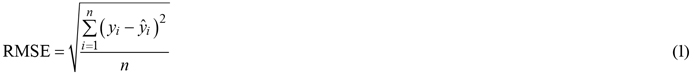
First, to get a better look into tree species proportions and the accuracy of the predictions, the RMSEs and biases of tree species proportions and classification results for main tree species were calculated. RMSEs were calculated as (Eq. 1)
and biases were calculated as (Eq. 2)
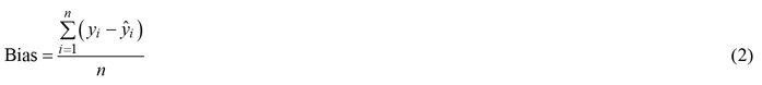
where n is the number of plots, yi is the ground truth value for plot i, ![]() is the predicted value for plot i using remote sensing data set. Relative RMSEs and biases were calculated by dividing RMSEs and biases with the average of the ground truth values and multiplying them by 100.
is the predicted value for plot i using remote sensing data set. Relative RMSEs and biases were calculated by dividing RMSEs and biases with the average of the ground truth values and multiplying them by 100.
The economic losses due to erroneous data were calculated for each plot using the operational large-scale forest planning system MELA (Hirvelä et al. 2017). MELA consists of two parts: (1) an automated stand simulator based on tree-level natural process (e.g. Hynynen et al. 2002) and production models (e.g. Kuitto et al. 1994) and 2) an optimisation package based on linear programming, JLP (Lappi 1992). Alternative treatment schedules were predicted with MELA using growing stock and site data as well as natural process and treatment models. The simulation time was 30 years with four periods (5-5-10-10 years). The first two five year periods originates from the planning periods’ lengths typically used in forest planning of private forests in Finland.
As we were interested in the economic losses due to the use of erroneous tree species proportions, the field plot data were used as true data. We maximised NPV at 1, 2, 3, 4 and 5 percent rates without any constraints to select optimal treatment schedules and assumed that these schedules were economically most profitable. Then, we optimised the treatment schedules using the four erroneous tree species proportion predictions, with accuracy levels resulting from the four remote sensing data sets. All optimisations were done by using JLP (Lappi 1992). Finally, we applied the obtained erroneous optimised schedules one by one with true data to see what were the true economic consequences of following them.
The MELA system simulates feasible predefined treatment schedules automatically for each plot based on the information available using built-in event routines and forest management recommendations (Äijälä et al. 2014; Vanhatalo et al. 2015), and the number of simulated schedules is limited. The simulation is guided through a large set of parameters. As a result from this, sometimes the set of schedule alternatives simulated for the plot from the true data did not include the optimal schedule, and a schedule selected with some erroneous data proved to be optimal. In such a case, we adopted that schedule as the true optimum, and after that the observed loss of that plot was zero (i.e. we did not accept negative losses).
We applied three analyses of the losses due to erroneous data. Firstly, we examined the losses caused by the errors in the tree species proportions. The errors of the proportions of the tree species came from the observed errors of the four remote sensing data sets, as we used predicted basal area proportions of the tree species. The generation of erroneous data of the plot has been introduced in Fig. 1. The total basal area of the plot was kept fixed, i.e. we assumed errors only in the species proportions. When species-wise basal area (and the respective number of stems) changed, also the basal-area weighted plot-level mean height and mean diameter (and the respective diameter and height distributions) changed in such plots in which there were at least two tree species. We also did one test with LIDAR2D data set, in which we calibrated diameter and height distributions so that the plot level (basal area weighted) mean diameter and mean height were fixed and the tree species level mean diameters and heights changed when the species proportions changed. For each method, we calculated the mean over all plots.
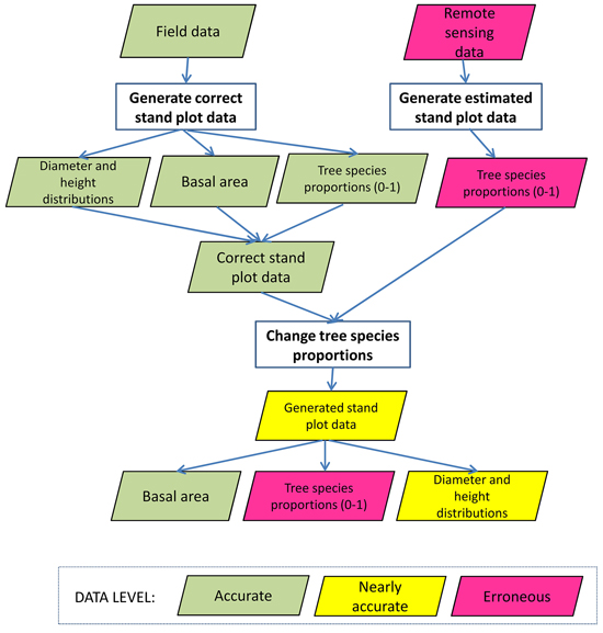
Fig. 1. Flow chart of the generation of the erroneous tree species proportions for each study plot. In the chart, green data box denotes that stand characteristics introduced in the box is accurate, yellow denotes it is nearly accurate and red box denotes it is erroneous.
Secondly, we examined the value of tree proportion information obtainable from the different remote sensing sources. For this, we needed a benchmark for comparison. We analysed how much more profit forest owner can get by using remote sensing data sets for estimating tree species proportions when compared to the situation in which tree species is random. To do this, we selected the tree species randomly for each tree stratum predicted with a given method for a given plot. Only one realisation of error was used, to produce counterpart to the results calculated in the first part.
The probability for selecting a given species was based on the tree species proportions of the study material, thus we assumed that we had prior information about the distributions of tree species proportions in the area. This reflects a situation where the tree species is estimated with remote sensing data, but where the remote sensing data do not explain any of the variation in the tree species. As in the previous case, we calculated the mean over all plots.
We calculated mean NPV losses in relation to the site type of the plots, and in relation to the maturity of the stands in plots based on classification used in Finland (Äijälä et al. 2014): Seedling stands are defined as having dominant height < 7 m (conifer) or 9 m (deciduous), and are often further divided into young (< 1.3 m) and advanced (1.3–7 or 9 m) seedling stands. Young thinning stands are defined as having basal area median diameter (Dgm) 8–16 cm and dominant height > 7 m (conifer) or 9 m (deciduous), and mean stand age at least 11 years and maximum 120 years in Southern Finland and 200 years in Northern Finland. Advanced thinning stands are defined as having Dgm over 16, and they are not yet classified as mature stands. Mean stand age is at least 25 years. Finally, mature stands are defined as stands, in which forest owner gets more benefit from regeneration than onwards growing.
Thirdly, we generated data including site type errors (Site Type) by using Monte Carlo simulation, because the site type was not interpreted from any data sets of our study. We used error levels of Lidar data observed from the study of Holopainen et al. (2010). Consequently, we generated 10 random errors of the site types with classification accuracy of 76% for pine-dominated forests and 69% for spruce- or birch-dominated plots for each plot, and that resulted 73.6% overall accuracy of site type classifications in Site Type data (Table 3). In this case we used several realisations, as the probability of correct site type classification is quite high, so that we would obtain at least one erroneous realisation for all stands.
| Table 3. The error matrix of Site type data (OMaT Very rich sites; OMT Rich sites; MT Damp sites; VT Sub-dry sites; CT Dry sites; ClT Barren sites; Rsa Rocky or sandy areas). | |||||||||
| Ground truth data | |||||||||
| OMaT | OMT | MT | VT | CT | ClT | Rsa | Total | ||
| Generated data | OMaT | 71 | 252 | 8 | 0 | 0 | 0 | 0 | 331 |
| OMT | 9 | 1164 | 894 | 7 | 0 | 0 | 0 | 2074 | |
| MT | 0 | 259 | 4632 | 865 | 6 | 0 | 0 | 5762 | |
| VT | 0 | 5 | 944 | 5226 | 273 | 1 | 0 | 6449 | |
| CT | 0 | 0 | 12 | 835 | 1597 | 7 | 0 | 2451 | |
| ClT | 0 | 0 | 0 | 7 | 249 | 96 | 13 | 365 | |
| Rsa | 0 | 0 | 0 | 0 | 5 | 16 | 57 | 78 | |
| Total | 80 | 1680 | 6490 | 6940 | 2130 | 120 | 70 | 17510 | |
To obtain a benchmark case as for the species data, we also simulated the site types for each plot randomly, i.e. purely based on the prior information of the distribution of the site type classes in the study data. In the case of site types, we calculated the mean over the stands and realisations.
3 Results
The tree species proportions were most accurate with LIDAR2D data set (Table 4). As pine was the dominant tree species approximately in two thirds of the plots in our data, the relative RMSEs of pine proportions were clearly smaller for each remote sensing data set than those of spruce or broad-leaved trees. Biases of the tree species proportions were smallest with LIDAR2D data set. Pine proportions were slightly underestimated and spruce and broad-leaved tree proportions overestimated, namely from 4.4% to 7.0%, 3.3% to 7.0% and 9.9% to 14.8%, respectively.
| Table 4. RMSEs and biases of the tree species proportions with four remote sensing data sets (relative RMSEs and biases are in the parenthesis). | ||||
| Data set | Pine, m2 ha–1 (%) | Spruce, m2 ha–1 (%) | Broad-leaved trees, m2 ha–1 (%) | |
| RMSE | LIDAR2D | 4.1 (39.1) | 4.1 (102.5) | 2.8 (91.4) |
| 2D | 5.1 (48.5) | 4.9 (122.3) | 3.3 (106.8) | |
| 3D2D | 5.0 (48.0) | 4.6 (114.8) | 3.1 (98.4) | |
| Satellite | 6.2 (59.5) | 5.4 (135.3) | 3.7 (117.5) | |
| Bias | LIDAR2D | –0.5 (–4.4) | 0.1 (3.3) | 0.3 (10.5) |
| 2D | –0.7 (–7.0) | 0.3 (6.7) | 0.5 (14.8) | |
| 3D2D | –0.6 (–6,1) | 0.3 (6.4) | 0.4 (12.3) | |
| Satellite | –0.6 (–5.6) | 0.3 (7.0) | 0.3 (9.9) | |
The classification of dominant tree species was quite accurate for pine-dominated plots with all four remote sensing data sets, whereas accuracy was quite modest for spruce or broad-leaved tree dominated plots with 2D, 3D2D and Satellite data set (Table 5). When the species proportions were assigned randomly, the dominant tree species classification accuracies were, as expected, clearly lower. In case of LIDAR2D, the dominant tree species classification result was improved by 23.2, for 2D data set by 21.39, for 3D2D by 21.5 and for satellite data set by 19.1 per cent units when compared to the random assignment. Although the spruce and broad-leaved tree plots were in general poorly classified, the LIDAR2D data set more than doubled the dominant tree species classification accuracy. This describes the maximal benefit obtainable from the remote sensing data.
| Table 5. Species-wise and overall classification accuracies of dominant tree species of four remote sensing data sets without and with randomisation of classifications of tree species proportions. | ||||
| Method | Pine (%) | Spruce (%) | Broad-leaved trees (%) | Total (%) |
| LIDAR2D | 91.0 | 49.3 | 51.6 | 78.9 |
| 2D | 91.4 | 41.9 | 38.1 | 76.0 |
| 3D2D | 92.5 | 35.6 | 37.7 | 75.6 |
| Satellite | 87.5 | 41.6 | 35.8 | 72.9 |
| Random, LIDAR2D | 69.9 | 21.6 | 23.5 | 55.7 |
| Random, 2D | 68.3 | 22.3 | 23.5 | 54.7 |
| Random, 3D2D | 68.2 | 17.7 | 25.5 | 54.1 |
| Random, satellite | 68.3 | 22.0 | 17.7 | 53.8 |
We optimised the treatments of the plots using the erroneous tree species proportions from the four remote sensing data sets. When these solutions were applied to the true data, they often proved to be sub-optimal solutions causing NPV losses. The losses were smallest with LIDAR2D data set (Table 6). The mean losses of the NPV at an interest rate of 3% varied from 124.4 € ha–1 to 167.7 € ha–1 for the 30 year period, depending on the data set.
| Table 6. Mean NPV losses (€ ha–1) for four remote sensing data sets at different interest rates. | ||||
| Interest rate | LIDAR2D | 2D | 3D2D | Satellite |
| 1% | 253.2 | 301.8 | 267.1 | 322.0 |
| 2% | 183.0 | 202.5 | 204.0 | 215.7 |
| 3% | 124.4 | 153.0 | 167.7 | 160.4 |
| 4% | 104.1 | 126.2 | 141.4 | 134.8 |
| 5% | 108.6 | 126.7 | 141.9 | 140.7 |
Mean NPV losses were a lot larger when we paid attention only to those plots in which sub-optimal treatment proposals were observed (Fig. 2). The proportions of such plots were quite remarkable, varying from 23.2% to 31.7%, depending on the remote sensing method and interest rate (Table 7). Relative losses increased clearly as interest rate increased. It was noticeable that the mean losses using the tree species proportions from 3D2D data were smaller than those obtained using 2D and Satellite data when smaller interest rates were used and then became larger with an interest rate of 3% or higher.
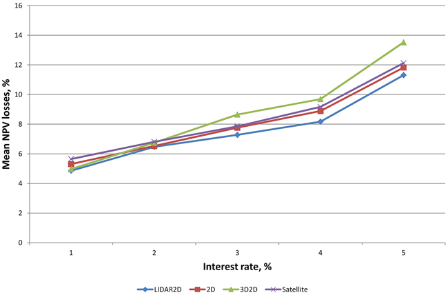
Fig. 2. Relative mean NPV losses at different interest rates.
| Table 7. Proportions of the plots with NPV losses at different interest rates. | ||||
| Plot proportions, % | ||||
| Interest rate, % | LIDAR2D | 2D | 3D2D | Satellite |
| 1 | 24.8 | 27.1 | 25.6 | 27.2 |
| 2 | 28.2 | 31.0 | 30.2 | 31.6 |
| 3 | 26.5 | 30.6 | 30.0 | 31.7 |
| 4 | 25.9 | 28.9 | 29.7 | 29.9 |
| 5 | 23.2 | 25.9 | 25.4 | 28.1 |
The more fertile the site type of the plot was the larger the mean losses were (Fig. 3). Mean losses were smallest in young thinning stands and largest in seedling and mature stands with interest rate of 3% (Fig. 4). It was noticeable that mean losses in mature stands with 3D2D data were clearly largest, and that mostly explains why overall losses were largest with 3D2D data at interest rate of 3%.
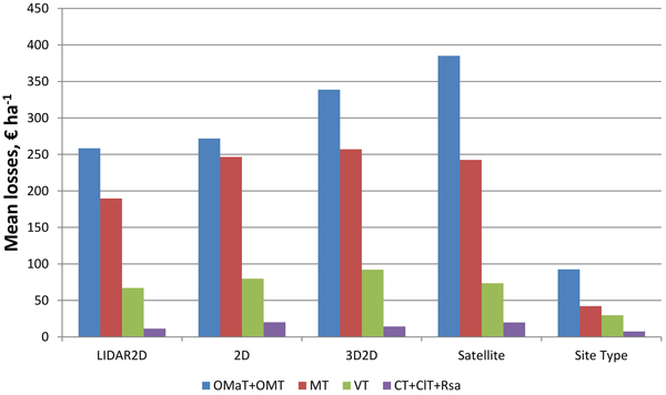
Fig. 3. Mean NPV losses of the plots at interest rate of 3% in relation to the site type of the plots, when species-wise proportion errors (LIDAR, 2D, 3D2D, Satellite) and site type errors (Site Type) are considered (OMaT Very rich sites; OMT Rich sites; MT Damp sites; VT Sub-dry sites; CT Dry sites; ClT Barren sites; Rsa Rocky or sandy areas).
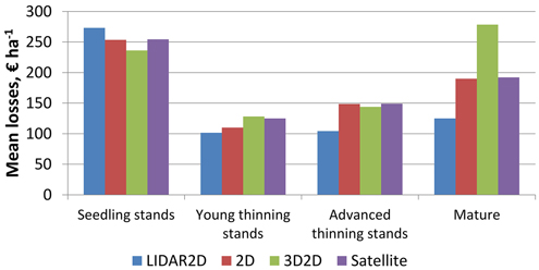
Fig. 4. Mean NPV losses of the plots at interest rate of 3% in relation to the maturity of the stands within the plots, when species-wise proportion errors are considered.
In few plots, species-wise number of stems changed noticeably, when the tree species proportions within the plot varied, but the mean diameter and height of the species were fixed. That also meant that at the plot level, the basal-area weighted mean diameter and height changed, as the proportions of the species changed. When the plot-level mean diameter and height were adjusted to the observed values and tree-species level diameters and heights were allowed to change, this further increased the losses by NPV 15 € ha–1 at interest rate of 3%.
When the errors of the tree species proportions were randomly simulated, the mean losses at interest rate of 3% increased to some extent (Table 8). On the other hand, the differences between the four remote sensing data sets diminished, as the only difference between the data sets was the number of tree species predicted to each plot. Thus, the monetary value of tree species data from remote sensing was 79.3, 53.3, 50.5 or 51 € ha–1 for LIDAR2D, 2D, 3D2D and satellite data set, respectively.
| Table 8. Mean losses of the randomised remote sensing inventory data sets and site type data for all plots and for plots with sub-optimal treatment proposals with each data set at interest rate of 3%. Proportions of the sub-optimally treated plots are in parenthesis. | ||
| Mean losses, all plots, € | Mean losses, sub-optimally treated plots, € (proportions in parenthesis) | |
| Random, LIDAR2D | 203.7 | 540.4 (35.9%) |
| Random, 2D | 206.3 | 520.1 (37.9%) |
| Random, 3D2D | 218.5 | 522.5 (39.6%) |
| Random, Satellite | 211.0 | 519.8 (37.5%) |
| Random, Site Type | 92.1 | 421.4 |
When true data with sub-optimal treatment schedules caused by random errors in site type were used in simulations, the losses in NPV were 37.8 € ha–1. There was no clear difference whether the site type of the plot was overestimated or underestimated (losses with overestimated plots were 132 € ha–1 and with underestimated plots 154 € ha–1).
When the errors of the site type were completely randomly simulated, mean losses were almost tripled, from 37.8 to 92.1 € ha–1.
4 Discussion
Traditionally, total stand volume has been the parameter of greatest interest in forestry. For instance, in Sweden and Norway the multi-source forest resources maps based on Lidar data do not present the tree species proportions at all, only the total volumes within the pixels (Kangas et al. 2018b). Based on the results of this study, the tree species proportions seem to be very important. The mean loss in a meta-analysis of previous studies has been 130.1 € ha–1 (Kangas et al. 2018a), meaning that the errors in tree species proportions can be even more important than the errors in the total volume. Islam et al. (2009) also observed that errors even in involving dominated tree species caused sub-optimal treatment schedules and further significant changes in the holding-level forest plans.
When the values of species proportion information of different remote sensing sources were calculated, the LIDAR2D data were the most valuable by far. In this case, where the total basal area was correct in all cases, this does not come from the improved estimate of total volume, but from the improved tree species information as such. It can also be seen from the dominant tree species assessments, where LIDAR2D were able to classify spruce as dominant species 38% better than 3D2D photogrammetric data set, and broad-leaved trees 37% better, respectively.
The satellite images used in this study can be interpreted as sunk costs, as they are produced for other purposes. Costs are only assumed for data that would not necessarily be collected for other purposes. The most expensive data, the Lidar data, cost about 5 € ha–1. The reduction of losses from satellite image to Lidar with interest rate of 3% was 36 € ha–1. This is for the 30 year period, so that for one year it is 1.2 € ha–1. So, if the Lidar data is used for 5 years or more, it is profitable to buy the Lidar data just for the improved tree species proportions, even if the other variables did not improve at all. As the losses are likely to decline in time due to discounting, the losses for the first five years are underestimated, which further increases the profitability of laser scanning for tree species information. For 2D aerial image data, the improvement was 7.4 € ha–1, so acquiring this data for 5 years would be profitable if the data would cost no more than 1.23 € ha–1. Compared to random tree species information, the profitability is obviously better.
Also, site index errors caused some economic losses, but not as high as the errors in the tree species. Yet, Eid (2000) noted that in the Norwegian context, the site index was the other most important variable besides age and the errors in the basal area did not cause losses at all. The explanation for this behaviour in the results is that the growth models in MELA system are sensitive to the species-wise basal areas, while the growth models in GAYA system used by Eid (2000) are most sensitive to the site index. Obviously, variables that have only a small effect on the growth predictions in the first place, cannot have large value as information.
In Eid (2000), the losses were low for the overmature stands. In our study, the losses were highest in the mature stands. Thus, in our data the mature stands were still growing so well that the immediate clear felling was not necessarily the best treatment schedule. Partly this may be due to the definition of mature in these studies, and partly due to the differences in the datasets, as in Eid (2000), the study data consist of spruce forests only. However, one possible explanation for the difference is again the differences between the growth models. In the Finnish models, age is not used as an explanatory variable.
In our study, the mean losses markedly decreased with increasing interest rate (but relative losses increased). We used NPV as the objective in the calculations and because of the economical objective, increasing the interest rate tends to push the cuttings to happen earlier. This may prevent economic losses as the optimal decision is less uncertain. When other objectives besides NPV, such as sustainable felling removal of stem wood or landscape management are applied in optimisation, the situation becomes more complex (e.g. Kangas et al. 2010).
Typically, impacts of uncertainty associated with inventory data are studied with propagated errors (Mäkinen et al. 2009, 2012; Kangas et al. 2018a). In these studies, usually the errors of the basal area, mean height and mean diameter of the tree species within stand are applied. In this study, we wanted to examine other potential error sources. To do this, we added only one error source at a time to the true data. However, it is impossible to change only the tree species proportions without also affecting other aspects of the data, such as the basal area weighted plot-level mean diameter and mean height, even though the total basal area was kept correct. This could have affected the economic losses observed in this study. On the other hand, calibrating the mean diameter and height to correct values at plot level slightly increased the already high losses observed.
It is likely that the errors in the different variables have interactions, and while an error in one variable may increase the losses, the errors in another variable could reduce the losses. Such interactions may explain the high losses given that only the tree species proportions were assumed erroneous. The analysis of such interactions remains to be studied in the future.
To get a better viewpoint of the utilisation of each remote sensing method, we also simulated the errors of the tree species proportions and site types randomly. In the random case, the differences between the mean losses of the tree proportions predicted from the four remote sensing data sets diminished. Compared to the random case, the mean losses decreased most with the LIDAR2D data, and least with Satellite data. If we only look at the plots where sub-optimal treatments were observed, mean losses were more or less at the same level with the data that included errors due to remote sensing and with data that included random errors. With 3D2D data set the mean losses were even a little higher compared to data with random errors. With random errors, the number of stands with economic losses was higher, but when the losses were observed, they were at a similar level. Thus, when the tree species is incorrect, the resulting losses are similar, irrespective of how the error occurred. This is because the number of treatment schedules considered is limited, and in each case one of this limited set of options is selected.
The economic losses denote how much more utility the forest owner could get by rescheduling the cuttings and other forest management operations. Regarding the forest owner, a new inventory or supplementing one can be worth it if new incomes from the forestry are greater than the increased inventory costs (Eyvindson et al. 2017).
Accurate tree species identification can be seen as one challenge of current operational forest inventory for acquiring data for private forest management planning in Finland. In the Finnish system, the tree species proportions usually result directly from the used k-nn estimation method (Packalen and Maltamo 2008). In other countries, the tree species may be obtained from visual inspection, even when remote sensing data is used to predict the volumes (e.g. Nilsson et al. 2017; Kangas et al 2018b). Accurate information on the tree species within a stand improves e.g. growth and yield predictions and treatment schedule suggestions, as well as upgrading estimates of cutting possibilities and removals. More accurate tree species proportion and site type data also help when trade-offs between timber production and some other ecosystem services like conservation prioritisation (e.g. Lehtomäki et al. 2015; Saarinen et al. 2018) are considered.
Acknowledgements
The authors wish to thank Ministry of Agriculture and Forestry key project “Puuta liikkeelle ja uusia tuotteita metsästä” for the financial support for this study.
References
Äijälä O., Koistinen A., Sved J., Vanhatalo K., Väisänen P. (eds.) (2014). Metsänhoidon suositukset. Metsätalouden kehittämiskeskus Tapion julkaisuja. 181 p. http://tapio.fi/wp-content/uploads/2015/06/Metsanhoidon_suositukset_ver3_netti_1709141.pdf. [Cited 24 Jan 2019]. [In Finnish].
Axelsson A., Lindberg E., Olsson H. (2018). Exploring multispectral ALS data for tree species classification. Remote Sensing 10(2): 183. https://doi.org/10.3390/rs10020183.
Birchler U., Bϋtler M. (2007). Information economics. Routledge advanced texts in economics and finance. Routledge, London. 462 p. ISBN 978-0415-37346-3.
Borders B.E., Harrison W.M., Clutter M.L., Shiver B.D., Souter R.A. (2008). The value of timber inventory information for management planning. Canadian Journal of Forest Research 38(8): 2287–2294. https://doi.org/10.1139/X08-075.
Burkhart H.E., Stuck R.D., Leuschner W.A., Reynolds M.A. (1978). Allocating inventory resources for multiple-use planning. Canadian Journal of Forest Research 8(1): 100–110. https://doi.org/10.1139/x78-017.
Duvemo K. (2009). The influence of data uncertainty on planning and decision processes in forest management. Ph.D. thesis. Department of Forest Resource Management, Faculty of Forest Sciences, SLU, Umeå. https://pub.epsilon.slu.se/1924/1/Duvemo_Avhandling_b.pdf. [Cited 18 Nov 2018]
Eid T. (2000). Use of uncertain inventory data in forestry scenario models and consequential incorrect harvest decisions. Silva Fennica 34(2): 89–100. https://doi.org/10.14214/sf.633.
Eyvindson K., Kangas A. (2014). Stochastic goal programming in forest planning. Canadian Journal of Forest Research 44(10): 1274–1280. https://doi.org/10.1139/cjfr-2014-0170.
Eyvindson K., Kangas A., Petty A. (2017). Determining the appropriate timing of the next forest inventory: incorporating forest owner risk preferences and the uncertainty of forest data quality. Annals of Forest Research 74: 2. https://doi.org/10.1007/s13595-016-0607-9.
Fassnacht F.A., Latifi H., Stereńczak K., Modzelewska A., Lefsky M., Waser L.T., Straubf C., Ghosh A. (2016). Review of studies on tree species classification from remotely sensed data. Remote Sensing of Environment 186: 64–87. https://doi.org/10.1016/j.rse.2016.08.013.
Haara A., Kangas A. (2019). Puulajivirheiden vaikutus puukauppatarjousten paremmuuden arvioimiseen sekä odotettujen ja toteutuvien tulojen eroihin sähköisessä tarjouskilpailutilanteessa. [Effect of tree species proportions errors to the comparison of purchase offers of timber sales agreements and differences between expected and actualised incomes in electronic bidding competition]. Metsätieteen aikakauskirja 2019-10079. 12 p. https://doi.org/10.14214/ma.10079. [In Finnish].
Haara A., Korhonen K.T. (2004). Kuviottaisen arvioinnin luotettavuus. [Accuracy of stand level mensuration]. Metsätieteen aikakauskirja 4/2004: 489–508. https://doi.org/10.14214/ma.5667. [In Finnish].
Hamilton D.A. (1978). Specifying precision in natural resource inventories. In: Integrated inventories of renewable resources: proceedings of the workshop. USDA Forest Service, General technical report RM-55: 276–281.
Hirvelä H., Härkönen K., Lempinen R., Salminen O. (2017). MELA2016 reference manual. Natural Resources Institute Finland (Luke). 547 p. http://urn.fi/URN:ISBN:978-952-326-358-1. [Cited 18 Nov 2018].
Holopainen M., Vastaranta M., Haapanen R., Yu X., Hyyppä J., Kaartinen H., Viitala R., Hyyppä H. (2010.) Site-type estimation using airborne laser scanning and stand register data. Photogrammetric Journal of Finland 22(1): 16–32. https://foto.aalto.fi/seura/julkaisut/pjf/pjf_e/2010/PJF2010_Holopainen_et_al.pdf. [Cited 17 Aug 2018]
Hotanen J.-P., Nousiainen H., Mäkipää R., Reinikainen A., Tonteri T. (2018). Metsätyypit – kasvupaikkaopas. [Guidebook of forest site types]. Metsäkustannus. 191 p. ISBN-13 9789523380486. [In Finnish].
Hynynen J., Ojansuu R., Hökkä H., Siipilehto J., Salminen H., Haapala P. (2002). Models for predicting stand development in MELA System. Finnish Forest Research Center, Research Papers 835. 116 p. http://urn.fi/URN:ISBN:951-40-1815-X. [Cited 12 Aug 2018].
Islam N., Kurttila M., Mehtätalo L., Haara A. (2009). Analyzing the effects of inventory errors on holding-level forest plans: the case of measurement error in the basal area of the dominated tree species. Silva Fennica 43(1): 71–85. https://doi.org/10.14214/sf.218.
Jansson G., Angelstam P. (1999). Threshold levels of habitat composition for the presence of long-tailed tit (Aegithalos audatus) in a boreal landscape. Landscape Ecology 14(3): 283–290. https://doi.org/10.1023/A:1008085902053.
Kangas A. (2010). Value of forest information. European Journal of Forest Research 129(5): 863–874. https://doi.org/10.1007/s10342-009-0281-7.
Kangas A., Horne P., Leskinen P. (2010). Measuring the value of information in multi-criteria decision making. Forest Science 56: 558–566.
Kangas A., Gobakken T., Puliti S., Hauglin M., Naesset E. (2018a). Value of airborne laser scanning and digital aerial photogrammetry data in forest decision making. Silva Fennica 52(1) article 9923. https://doi.org/10.14214/sf.9923.
Kangas A., Astrup R., Breidenbach J., Fridman J., Gobakken T., Korhonen K.T., Maltamo M., Nilsson M., Nord-Larsen T., Næsset E., Olsson H. (2018b). Remote sensing and forest inventories in Nordic countries – roadmap for the future. Scandinavian Journal of Forest Research 33(4): 397–412. https://doi.org/10.1080/02827581.2017.1416666.
Kokkoniemi S. (2012). Laserkeilaukseen ja metsäsuunnittelutietoon perustuvan pituusbonitoinnin tarkkuus. [Accuracy of site index derived by airborne laser scanning and stand register data]. The Department of Forest Sciences, University of Helsinki. 53p + appendices. http://urn.fi/URN:NBN:fi:hulib-201507211949. [Cited 15 Nov 2018]. [In Finnish].
Korpela I., Koskinen M., Vasander H., Holopainen M., Minkkinen K. (2009). Airborne small-footprint discrete-return LiDAR data in the assessment of boreal mire surface patterns, vegetation and habitats. Forest Ecology and Management 258(7): 1549–1566. https://doi.org/10.1016/j.foreco.2009.07.007.
Kuitto P.-J., Keskinen S., Lindroos J., Oijala T., Rajamäki J., Räsänen T., Terävä J. (1994). Puutavaran koneellinen hakkuu ja metsäkuljetus. [Mechanical felling and forest haulage of timber]. Metsätehon tiedotus 410. [In Finnish].
Kukkonen M., Korhonen L., Maltamo M., Suvanto A., Packalen P. (2018). How much can airborne laser scanning based forest inventory by tree species benefit from auxiliary optical data? International Journal of Applied Earth Observations and Geoinformation 72: 91–98. https://doi.org/10.1016/j.jag.2018.06.017.
Laine J., Vasander H., Hotanen J.-P., Nousiainen H., Saarinen M., Penttilä T. (2018). Suotyypit ja turvekankaat – kasvupaikkaopas. [Forest peatland and heathy peatland types-classification guide]. Metsäkustannus Oy. 160 p. ISBN-13 978-952-5694-89-5.
Lappi J. (1992). JLP: a linear programming package for management planning. Finnish Forest Research Institute, Research Papers 414. 134 p. http://urn.fi/URN:ISBN:951-40-1218-6.
Lehtomäki J., Tuominen S., Leinonen A. (2015). What data to use for forest conservation planning? A comparison of coarse open and detailed proprietary forest inventory data in Finland. PLoS ONE 10(8): e0135926. https://doi.org/10.1371/journal.pone.0135926.
Mäkinen A., Holopainen M., Kangas A., Rasinmäki J. (2009). Propagating the errors of initial forest variables through stand- and tree-level growth simulators. European Journal of Forest Research 129(5): 887–897. https://doi.org/10.1007/s10342-009-0288-0.
Mäkinen A., Kangas A., Nurmi M. (2012). Using cost-plus-loss analysis to define optimal forest inventory interval and forest inventory accuracy. Silva Fennica 46(2): 211–226. https://doi.org/10.14214/sf.55.
Maltamo M., Packalen P. (2014). Species-specific management inventory in Finland. In: Maltamo M., Næsset E,, Vauhkonen J. (eds.). Forestry applications of airborne laser scanning – concepts and case studies. Managing Forest Ecosystems, vol 27. Springer, Dordrecht. p. 241–252. https://doi.org/10.1007/978-94-017-8663-8_12.
Maltamo M., Eerikäinen K., Pitkänen J., Hyyppä J., Vehmas M. (2004). Estimation of timber volume and stem density based on scanning laser altimetry and expected tree size distribution functions. Remote Sensing of Environment 90(3): 319–330. https://doi.org/10.1016/j.rse.2004.01.006.
Næsset E. (2002). Predicting forest stand characteristics with airborne scanning laser using a practical two-stage procedure and field data. Remote Sensing of Environment 80(1): 88–99. https://doi.org/10.1016/S0034-4257(01)00290-5.
Næsset E. (2004). Accuracy of forest inventory using airborne laser scanning: evaluating the first Nordic full-scale operational project. Scandinavian Journal of Forest Research 19(6): 554–557. https://doi.org/10.1080/02827580410019544.
Nilsson M., Nordkvist K., Jonzén J., Lindgren N., Axensten P., Wallerman J., Egberth M., Larsson S., Nilsson L., Eriksson J., Olsson H. (2017). A nationwide forest attribute map of Sweden predicted using airborne laser scanning data and field data from the National Forest Inventory. Remote Sensing of Environment 194: 447–454. http://dx.doi.org/10.1016/j.rse.2016.10.022.
Noordermeer L., Bollandsås O.M., Gobakken T., Næsset E. (2018). Direct and indirect site index determination for Norway spruce and Scots pine using bitemporal airborne laser scanner data. Forest Ecology and Management 428: 104–114. https://doi.org/10.1016/j.foreco.2018.06.041.
Ørka H.O., Hauglin M. (2016). Use of remote sensing for mapping of non-native conifer species. INA Fagrapport 33. 76 p. https://static02.nmbu.no/mina/publikasjoner/mina_fagrapport/pdf/mif33.pdf. [Cited 28 Aug 2018].
Ørka H.O., Næsset E., Bollandsås M. (2009). Classifying species of individual trees by intensity and structure features derived from airborne laser scanner data. Remote Sensing of Environment 113(6): 1163–1174. https://doi.org/10.1016/j.rse.2009.02.002.
Ørka H.O., Dalponte M., Gobakken T., Næsset E., Ene L.T. (2013). Characterizing forest species composition using multiple remote sensing data sources and inventory approaches. Scandinavian Journal of Forest Research 28(7): 677–688. https://doi.org/10.1080/02827581.2013.793386.
Packalén P., Maltamo M. (2008). Estimation of species-specific diameter distributions using airborne laser scanning and aerial photographs. Canadian Journal of Forest Research 38(7): 1750–1760. https://doi.org/10.1139/X08-037.
Packalén P., Suvanto A., Maltamo M. (2009). A two stage method to estimate species-specific growing stock. Photogrammetric Engineering & Remote Sensing 75(12): 1451–1460. https://doi.org/10.14358/PERS.75.12.1451.
Persson M. (2018). Tree species classification using multi-temporal Sentinel-2 data. Department of Forest Resource Management, Swedish University of Agricultural Sciences. 41 p. https://stud.epsilon.slu.se/13740/1/Persson_M_180726.pdf. [Cited 10 Oct 2018]
Saarinen N., Vastaranta M., Näsi R., Rosnell T., Hakala T., Honkavaara E., Wulder M.A., Luoma V., Tommaselli A.M.G., Imai N.N., Ribeiro E.A.W., Guimarães R.B., Holopainen M., Hyyppä H. (2018). Assessing biodiversity in boreal forests with UAV-based photogrammetric point clouds and hyperspectral imaging. Remote Sensing 10(2): 338. https://doi.org/10.3390/rs10020338.
Shang X., Chisholm L.A. (2014). Classification of Australian native forest species using hyperspectral remote sensing and machine-learning classification algorithms. IEEE Journal of Selected Topics in Applied Earth Observations and Remote Sensing 7(6): 2481–2489. https://doi.org/10.1109/JSTARS.2013.2282166.
Stoffels J., Hill J., Sachtleber T., Mader S., Buddenbaum H., Stern O., Langshausen J., Dietz J., Ontrup G. (2015). Satellite-based derivation of high-resolution forest information layers for operational forest management. Forests 6(6): 1982–2013. https://doi.org/10.3390/f6061982.
Tomppo E., Kuusinen N., Mäkisara K., Katila M., McRoberts R.E. (2016). Effects of field plot configurations on the uncertainties of ALS-assisted forest resource estimates. Scandinavian Journal of Forest Research 32(6): 488–500. https://doi.org/10.1080/02827581.2016.1259425.
Tuominen S., Pitkänen T., Balazs A., Kangas A. (2017). Improving Finnish Multi-Source National Forest Inventory by 3D aerial imaging. Silva Fennica 51(4) article 7743. https://doi.org/10.14214/sf.7743.
Vanhatalo K., Väisänen P., Joensuu S., Sved J., Koistinen A., Äijälä O. (eds.) (2015). Metsänhoidon suositukset suometsien hoitoon, työopas. Tapion julkaisuja. http://tapio.fi/wp-content/uploads/2015/06/MHS_opas_suometsien_hoitoon_20150222_TAPIO1.pdf. [Cited 24 Jan 2019]. [In Finnish].
White J.C., Coops N.C., Wulder M.A., Vastaranta M., Hilker T., Tompalski P. (2016). Remote sensing technologies for enhancing forest inventories: a review. Canadian Journal of Remote Sensing 42(5): 61–641. https://doi.org/10.1080/07038992.2016.1207484.
Willighagen E., Ballings M. (2015). genalg: R based genetic algorithm. https://cran.r-project.org/web/packages/genalg/index.html. [Cited 20 Nov 2018].
Total of 52 references.
