Hans Ole Ørka  ,
Endre H. Hansen,
Michele Dalponte,
Terje Gobakken,
Erik Næsset
,
Endre H. Hansen,
Michele Dalponte,
Terje Gobakken,
Erik Næsset
Large-area inventory of species composition using airborne laser scanning and hyperspectral data
Ørka H. O., Hansen E. H., Dalponte M., Gobakken T., Næsset E. (2021). Large-area inventory of species composition using airborne laser scanning and hyperspectral data. Silva Fennica vol. 55 no. 4 article id 10244. https://doi.org/10.14214/sf.10244
Highlights
- A methodology for using hyperspectral data in the area-based approach is presented
- Hyperspectral data produced satisfactory results for species composition in 90% of the cases
- Parametric Dirichlet regression is an applicable method to predicting species proportions
- Normalization and a tree-based selection of pixels provided the overall best results
- Both visible to near-infrared and shortwave-infrared sensors gave acceptable results.
Abstract
Tree species composition is an essential attribute in stand-level forest management inventories and remotely sensed data might be useful for its estimation. Previous studies on this topic have had several operational drawbacks, e.g., performance studied at a small scale and at a single tree-level with large fieldwork costs. The current study presents the results from a large-area inventory providing species composition following an operational area-based approach. The study utilizes a combination of airborne laser scanning and hyperspectral data and 97 field sample plots of 250 m2 collected over 350 km2 of productive forest in Norway. The results show that, with the availability of hyperspectral data, species-specific volume proportions can be provided in operational forest management inventories with acceptable results in 90% of the cases at the plot level. Dominant species were classified with an overall accuracy of 91% and a kappa-value of 0.73. Species-specific volumes were estimated with relative root mean square differences of 34%, 87%, and 102% for Norway spruce (Picea abies (L.) Karst.), Scots pine (Pinus sylvestris L.), and deciduous species, respectively. A novel tree-based approach for selecting pixels improved the results compared to a traditional approach based on the normalized difference vegetation index.
Keywords
airborne laser scanning;
Dirichlet regression;
hyperspectral;
species proportions;
species-specific forest inventory
-
Ørka,
Norwegian University of Life Sciences, Faculty of Environmental Sciences and Natural Resource Management, P.O. Box 5003, NO-1432 Ås, Norway
 https://orcid.org/0000-0002-7492-8608
E-mail
hans-ole.orka@nmbu.no
https://orcid.org/0000-0002-7492-8608
E-mail
hans-ole.orka@nmbu.no
-
Hansen,
Norwegian University of Life Sciences, Faculty of Environmental Sciences and Natural Resource Management, P.O. Box 5003, NO-1432 Ås, Norway; Norwegian Forest Extension Institute, Honnevegen 60, NO-2836 Biri, Norway
https://orcid.org/0000-0001-5174-4497
E-mail
eh@skogkurs.no
-
Dalponte,
Department of Sustainable Agro-ecosystems and Bioresources, Research and Innovation Centre, Fondazione E. Mach, Via E. Mach 1, 38010 San Michele all’Adige, TN, Italy
https://orcid.org/0000-0001-9850-8985
E-mail
michele.dalponte@fmach.it
-
Gobakken,
Norwegian University of Life Sciences, Faculty of Environmental Sciences and Natural Resource Management, P.O. Box 5003, NO-1432 Ås, Norway
https://orcid.org/0000-0001-5534-049X
E-mail
terje.gobakken@nmbu.no
- Næsset, Norwegian University of Life Sciences, Faculty of Environmental Sciences and Natural Resource Management, P.O. Box 5003, NO-1432 Ås, Norway E-mail erik.naesset@nmbu.no
Received 10 September 2019 Accepted 23 August 2021 Published 26 August 2021
Views 91210
Available at https://doi.org/10.14214/sf.10244 | Download PDF

1 Introduction
During the last two decades, stand-level forest management inventories (FMI) have been highly automated using remotely sensed data. In particular, airborne laser scanning (ALS) has improved the accuracy and efficiency of forest inventories used for management decisions at stand-level (Næsset 2002; Eid et al. 2004). Furthermore, the use of ALS enables the prediction of stand-level forest attributes such as stem volume, tree heights, stem diameters, basal area, and the number of stems over large areas with high accuracy (Maltamo and Packalen 2014; Næsset 2014). However, stand classification, i.e., the determination of site quality and species compositions are often provided by manual photo-interpretation (Næsset 2014). Automated methods based on remotely sensed data could be useful in providing these attributes, reducing the overall inventory costs. Information on tree species composition is particularly wanted as it is essential for predicting site quality (Kandare et al. 2017b) and as it represents the basis for the stratification used in ALS based inventories (Næsset and Gobakken 2008). Moreover, tree species information is frequently used as a biodiversity indicator (Gao et al. 2014; Kovac et al. 2020). In addition, tree species composition is of crucial importance to reduce erroneous management decisions and economic losses based on these decisions (Haara et al. 2019).
The importance of providing information about tree species in FMIs is reflected in the remote sensing literature as well. During the last decade, the number of scientific studies focusing on tree species classification has doubled (Fassnacht et al. 2016). However, on an operational basis, at least in Norway, little has changed regarding the methods used over the last three decades. The reasons behind this are likely many. Fassnacht et al. (2016) pointed out that the majority of these scientific studies only focus on small experimental areas and that species-specific inventories over large geographic extents are one of the most prominent challenges in the field of species classification. The lack of scientific evidence for accurate tree species classification over large areas likely limits the utility of developed inventory methods in operational projects.
Another factor limiting the utility of methods developed for species classification is the spatial level on which the studies have been conducted; much of the research on tree species classification is at individual tree crown level (Fassnacht et al. 2016). Classifying individual trees is usually straightforward as there is a one-to-one relationship between the object of interest and the class (Holmgren et al. 2008; Ørka et al. 2012; Dalponte et al. 2013). A significant drawback of an individual tree approach is that attributes at stand-level will be underestimated when aggregating individual trees volume by tree species since not all trees are detected in remotely sensed data (Persson et al. 2002; Dalponte et al. 2015; Kandare et al. 2017a). Thus, individual tree approaches have the risk of providing serious systematic errors, and area-based approaches will be the preferable choice (Coomes et al. 2017). Furthermore, supervised individual tree species classification methods require measurements of tree positions in the field. Measuring tree positions is labor-intensive, costly, and will influence current field protocols used in operational FMIs. Thus, an automated method following the area-based approach, while not increasing field costs or altering current field protocols, is desired.
In contrast to the one-to-one relationship between object and class, which we find in the individual tree approach, the relationship in the area-based approach is many-to-one, where for one sample plot there is a mix of trees with different species and sizes. Thus, species composition in area-based inventories can be provided as species-specific volumes (Peuhkurinen et al. 2008; Packalén et al. 2009), species-specific diameter distributions (Packalén and Maltamo 2008), species proportions of volume (Puliti et al. 2017a), species proportions of basal area (Ørka et al. 2013), or other species-specific forest attributes. The dominant species can also be classified directly (Mora et al. 2010). In Norway, the tradition is to provide the species proportions of volume.
Predicting species-specific attributes directly is a common approach in operational FMIs in Finland (Maltamo and Packalen 2014). The methods developed and used in Finnish FMIs utilize non-parametric techniques and provide species-specific forest attributes. The use of non-parametric nearest neighbor methods provides consistency between the predicted forest attributes. However, non-parametric methods usually require a large number of sample plots for training. In inventories adopting non-parametric practices, approximately 500 sample plots are used in young to mature forest stands (Maltamo and Packalen 2014). Similarly, when parametric approaches are used, 120–200 sample plots per inventory are measured depending on the number of strata (40–50 sample plots per strata) (Næsset 2014), and many ALS-based FMIs are based on such methods. Thus, alternatives to the non-parametric methods for providing species information are desired when the number of sample plots is limited. Logistic regression (Donoghue et al. 2007) and beta regression (Vihervaara et al. 2015) have been used to estimate species proportions in the two-species case. When extending to more than two species, Dirichlet regression (DR) is a common technique for estimating compositional data (e.g., Hijazi and Jernigan 2009; Morais et al. 2017). Puliti et al. (2017a) used DR to predict tree species proportions from variables derived from photogrammetric point clouds. Based on the combination of species proportions predicted using the DR and the total volume predicted separately, Puliti et al. (2017a) calculated species-specific volume estimates. DR has limitations on single-species plots, and for such situations, a small error is introduced (Maier 2014). The two-step procedure by Puliti et al. (2017a) models total volume and species proportions independently and provides consistency between predicted species-specific volumes, species proportions and dominant species, which is crucial.
The most discriminative remotely sensed data collected by airborne sensors for tree species classification are undoubtedly hyperspectral data. Fassnacht et al. (2016) reviewed more than 100 studies and found that the average accuracy of hyperspectral data was better than the one obtained using alternative data types. In the boreal forest, it is clear that hyperspectral data are among the most favorable data sources for separating tree species in terms of accuracy (Ørka et al. 2013; Dalponte et al. 2013). Hyperspectral data can differentiate between species because they provide detailed information on the spectral properties of tree canopies (Hovi et al. 2017). The few experimental studies investigating the use of hyperspectral data and the area-based approach (Ørka et al. 2013) also indicate that hyperspectral data are superior to other types of remotely sensed data for predicting tree species composition. However, no large-area inventory experiments have documented the accuracy that could be obtained with hyperspectral data in boreal forests. In large-area aerial data acquisition campaigns where ALS and hyperspectral data are acquired simultaneously, georeferencing, image quality, and reflectance problems arise. Vaglio Laurin et al. (2016), for instance, reported a georeferencing mismatch of 1–4 m between ALS data and hyperspectral imagery. Furthermore, data acquisition will span a longer time, and imagery will be collected during the entire day and maybe over many days. In a large-area FMI, such errors cannot be mitigated to the same extent as in small experimental studies where manual adjustments are sometimes performed to correct a geographical mismatch between the data. Therefore, it is of current interest to evaluate the suitability of hyperspectral data to provide species composition in operational FMIs.
Separating pixels from ground vegetation and tree crowns using different thresholds are found to be essential for individual tree classification (Dalponte et al. 2014). The conventional methods for thresholding hyperspectral images, when used in combination with ALS for forest application, includes a threshold based on an ALS-derived canopy height model or a spectral threshold. Dalponte et al. (2014) tested these methods for individual tree species classification and compared them to the use of all pixels (i.e., no thresholding) within the objects. They concluded that thresholding was important, but not all thresholding methods improved the classification. However, they suggested applying spectral thresholding. The evaluation of such thresholding in area-based inventories is limited. In addition to thresholding, preprocessing such as normalization of spectral values, has been applied for individual trees (Dalponte et al. 2013).
In studies of tree species classification using hyperspectral sensors, reports on the importance of the different wavelengths help us understand the data and the different spectral signals concerning the absorption features in plant pigments, water, and soil (Fassnacht et al. 2016). Analyses of which wavelengths are important for predicting species composition following the area-based approach in boreal forests are essential to guide the selection of hyperspectral sensors suitable for use in FMIs.
The overall objective of the current study was to develop and assess an area-based approach using hyperspectral data to predict tree species composition in an operational large-area FMI. The species composition results were evaluated as dominant species, species proportions, and species-specific volumes. The specific objectives were to:
1. evaluate effects of thresholding and normalization as preprocessing methods of hyperspectral data applied prior to computing variables for area-based inventories;
2. evaluate the influence of two different sensors operating in VNIR (visible and near-infrared) and SWIR (shortwave-infrared) ranges of the spectrum;
3. evaluate the important hyperspectral wavelengths for area-based prediction of species composition.
2 Material and methods
2.1 Study area
The study area covers approximately 350 km2 of productive forest land, located in the municipalities of Gran, Lunner, and Jevnaker in Norway (60°41´N, 10°45´E, 115–812 m above sea level, Fig. 1). The forest is dominated by Norway spruce (Picea abies (L.) Karst.) in moist and highly productive sites and Scots pine (Pinus sylvestris L.) in drier sites with lower productivity. Deciduous species, mainly birch (Betula spp.), can be found interspersed in sites dominated by conifers as well as in small patches.
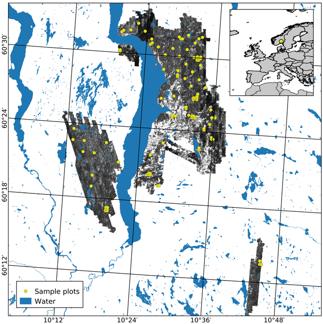
Fig. 1. The geographical location of the study area in Norway (insert) and the extent of the hyperspectral acquisition are shown using an image from the NIR band (708 nm). Sample plots appear in yellow.
2.2 Field data
The field data were combined from two datasets gathered for the purpose of an operational FMI and as part of a research project (see Puliti et al. 2017b for details). Summaries of the field data overlapping the study area and used in this study appear in Table 1 and Table 2. The operational FMI dataset was collected from May to November 2016. The sample plots were established in clusters distributed on a 1.5 × 1.5 km north/south grid. In each cluster, nine plots of 250 m2 were distributed on a 250 × 250 m grid. Plots in young forest areas or located outside the forest were not measured. The research dataset was collected in August and September of 2015. Sample plots were distributed on a 1.7 × 1.7 km south-east/north-west grid. The plot size was initially 500 or 1000 m2. However, the distance from the plot center to each tree was measured using a total station. The distance measurements were used to identify trees within a radius corresponding to a plot size of 250 m2.
| Table 1. Summary of volume and species proportions on the 97 sample plots used for training and validation for Spruce (Picea abies), Pine (Pinus sylvestris), Deciduous species (mainly birch (Betula spp.)) and in total. Mean values for all plots are presented in parenthesis. | ||
| Species | Species proportion, (mean) (%) | Volume, (mean) in m3 ha–1 |
| Spruce | 1–100 (67) | 1–625 (168) |
| Pine | 0–98 (21) | 0–369 (48) |
| Deciduous | 0–83 (12) | 0–155 (25) |
| Total | 16–625 (241) | |
| Table 2. Summary of number of plots, percent of dominant species of total plot volume and volume for training and validation plots by dominant species; Spruce-dominated (Picea abies), Pine-dominated (Pinus sylvestris), Deciduous-dominated (mainly dominated by Birch (Betula spp.)) and in total. Mean values for all plots are presented in parenthesis. | |||
| Dominant species | Number of plots | % of dominant species of total plot volume (mean) | Volume, (mean) in m3 ha–1 |
| Spruce-dominated | 70 | 45–100 (85) | 24–625 (257) |
| Pine-dominated | 22 | 39–98 (71) | 65–471 (227) |
| Deciduous-dominated | 5 | 53–83 (68) | 16–266 (129) |
| Total | 97 | 16–625 (241) | |
For each plot, species and diameter at breast height (DBH) were recorded for trees with DBH ≥ 6 cm. Tree heights were measured on approximately 10 sample trees per plot using a Vertex hypsometer. The sample trees were selected with probability proportional to stem basal area. From these measurements, total and species-specific volume were obtained using the following approach. First, the volume of each tree was calculated using the observed DBH and a tree height obtained by applying a stand height curve model (Fitje and Vestjordet 1977) and standard Norwegian allometric volume models (Braastad 1966; Brantseg 1967; Vestjordet 1967). Afterward, the “true” volume was estimated using the mean-of-rations estimator (eg., Avery and Burkhart 2015). The ratio that adjusts the modeled volumes to “true” volumes was calculated plot- and species-wise from the sample trees as the mean ratio between “true” sample tree volume (using the observed height) and the modeled volume (using the stand height curve model). Stratum- and species-wise ratios were applied if there were less than three trees of a specific species on a plot.
2.3 Remotely sensed data
2.3.1 Airborne laser scanning
ALS data were acquired using a Leica ALS70 sensor on May 2–10 and June 11–20, 2015. The data were acquired with a fixed-wing aircraft flying at an altitude of 1100 m above ground level at a speed of 77 m s–1. The ALS sensor was operated at a pulse repetition frequency of 273 kHz and a scan angle of ±18 degrees. Initial processing of the data was performed by the contractor (Terratec AS, Norway). This included computation of planimetric coordinates, ellipsoid height values, and classification of echoes into ground and non-ground according to the proprietary algorithm implemented in Terrascan software (Soininen 2016). Up to six echoes per pulse were recorded, and the resulting density of first echoes on the sample plots was 15.0 m–2.
ALS echoes were categorized as “single,” “first of many,” “intermediate,” and “last of many”. “Single” and “first of many” were merged into one dataset and denoted as “first,” whereas the “last of many” echoes constituted one dataset denoted as “last”. Less than 6% of the echoes were in the “Intermediate” echo category. These echoes were discarded to comply with operational FMI methods. From the ALS echoes in each of the two categories (“first”, “last”), variables describing the height and density of the vegetation were derived. For each plot, canopy height variables, including percentiles at 10% intervals (H10, H20, …, H90), were derived from laser echoes above a threshold of 1.3 m above ground. Furthermore, canopy density variables were computed by first dividing the range between a 95% percentile height and the 1.3 m threshold into ten vertical layers of equal height. The proportion of echoes above each layer to the total number of echoes were computed, resulting in ten canopy density variables (D0, D1, …, D9). In addition, maximum height (Hmax), mean height (Hmean), standard deviation (Hsd), and coefficient of variation (Hcv) were computed for echoes above the threshold.
2.3.2 Hyperspectral imagery
Hyperspectral data were acquired using the Compact Airborne Spectrographic Imager (CASI, model 1500h) and the Shortwave infrared Airborne Spectrographic Imager (SASI, model 1000A) from ITRES Research Limited, Canada. The CASI sensor covered the visible and near-infrared parts of the spectrum from 367 nm to 1045 nm with a spectral resolution of 9.4 nm, while the SASI sensor covered the short-wavelength infrared parts from 957 nm to 2443 nm with a spectral resolution of 15 nm.
The acquisition was conducted on August 21–22, 2015, using a fixed-wing aircraft flying at an altitude of approximately 1500 m above ground level. The equipment platform in the aircraft was not gyro stabilized. In total, data along 69 flight lines were acquired during the two days. The acquisition settings resulted in 72 channels with a spatial resolution of 0.5 m for the CASI sensor and 100 channels with 1 m spatial resolution for the SASI sensor. The images were acquired between 10:09 AM and 15:41 PM local time (CEST), having a zenith angle between 24° and 40° and azimuth ranging from 158° to 252° and thus providing significant variation in acquisition conditions. The solar noon was at 1:18 PM and 77 sample plots were within a ±2-hour interval from the solar noon.
2.3.3 Preprocessing of hyperspectral imagery
Two preprocessing steps were used to derive the hyperspectral variables: a data normalization and a pixel thresholding. Data normalization was carried out by scaling the band pixel values relative to the sum of all band values within the pixel (Yu et al. 1999). Pixel thresholding was done selecting the pixels inside each sample plot before computing variables (Dalponte et al. 2014). Both preprocessing steps were used previously in literature and they showed to be useful in reducing the discrepancies among the hyperspectral stripes (normalization), and to reduce the noise due to the potential georeferencing errors among the ALS and hyperspectral geometries (pixels thresholding). In both cases we considered multiple options. Regarding the data normalization two options were explored: i) normalized dataset, and ii) raw dataset without normalization. Concerning the pixel thresholding three options were explored: i) no thresholding; ii) NDVI thresholding; and iii) tree-based (TB) thresholding. In the no thresholding option all pixels were kept into the analysis. The normalized difference vegetation index (NDVI) (Haboudane et al. 2004) thresholding consisted in selecting only pixels with NDVI above 0.5 to compute the variables as used in other species-specific prediction studies (Dalponte et al. 2008; Kandare et al. 2017a). The NDVI mask was resampled to carry out the thresholding on the SASI sensor. The last thresholding was a new tree-based (TB) thresholding method. A simple segmentation algorithm was applied to the hyperspectral images and the delineated “tree crowns” were used to select pixels to be used in the statistical modeling. Segmentation on the hyperspectral imagery was preferred over an ALS derived canopy height model due to the potential georeferencing errors. The TB segmentation was based on the CASI band 552 nm. First, a Gaussian filter with one sigma was applied. A mask was created by first applying Otsu histogram thresholding (Otsu 1979) and further filtering the mask using a circular disk of 2 pixels. A maximum filter of 3 by 3 pixels was applied to find treetops (local maxima) which were used as markers in a marker-based watershed algorithm. From the pixels selected using thresholding, the mean value in each band was computed and used in the modeling. Furthermore, we computed six different vegetation indices (Table 3). This resulted in a total of 78 variables from the CASI sensor and 100 from the SASI sensor for each combination of normalization and thresholding. Thus, the variables used to model species composition were based on the combination of normalization and thresholding in a crossed design (Fig. 2), thus six different combinations of preprocessing methods were evaluated (Fig. 3):
● no normalization and no thresholding (RAWNO);
● no normalization and NDVI thresholding (RAWNDVI);
● no normalization and TB thresholding (RAWTB );
● normalization and no thresholding (NORMNO );
● normalization and NDVI thresholding (NORMNDVI);
● normalization and TB thresholding (NORMTB).
| Table 3. Computation and reference for vegetation indices derived from hyperspectral data and applied in the modelling of species composition. | ||
| Index | Computation | Reference |
| Normalized Difference Vegetation Index | Rouse et al. (1973) | |
| Renormalized Difference Vegetation Index | Roujean and Breon (1995) | |
| Modified red edge Simple Ratio index | Chen (1996) | |
| Conifer Index | Trier et al. (2018) | |
| Spruce Index | Trier et al. (2018) | |
| Soil-Adjusted Vegetation Index | Huete (1988) | |
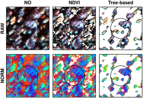
Fig. 2. Example from one field plot applying different normalization (RAW, NORM) and thresholding approaches (NO, NDVI, tree-based). Pixels removed applying thresholding appear white and are not used when computing variables for modelling. Image colors: red = 445 nm, green=714 nm, and blue=839 nm using a linear stretch.
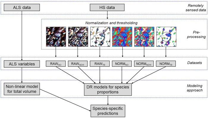
Fig. 3. Schematic diagram of the data processing and modeling steps used in the study. From the remotely sensed data preprocessing is applied to the hyperspectral (HS) data in terms of normalization and thresholding, providing six different datasets for Dirichlet (DR) modelling of species proportions; RAWNO (no normalization and no thresholding), RAWNDVI (no normalization and NDVI thresholding), RAWTB (no normalization and tree-based (TB) thresholding), NORMNO (normalization and no thresholding), NORMNDVI (normalization and NDVI thresholding), and NORMTB (normalization and TB thresholding). Variables from airborne laser scanning (ALS) data are used in modeling of total volume.
2.4 Modeling and validation
The modeling of the tree species composition was performed in three steps. First, the total volume was modeled using ALS data. Next, the species proportions were modeled using hyperspectral data. Finally, species-specific volumes and dominant species according to volume were established based on the species proportions predicted. Species-specific volumes were established by multiplying the total volume by the species proportions and the species with the largest volume was assigned as the dominant species. All steps were included in a ten-fold cross-validation. This procedure was performed for all combinations of normalization and thresholding applied to the hyperspectral data prior to extracting variables. Also, results for the two sensors, CASI and SASI, and the two combined, were assessed.
2.4.1 Predicting total volume using non-linear regression
The relationships between the total volumes and the ALS variables were modeled using non-linear regression with both dependent and independent variables at the original scale. The models were of the form displayed in Eq. 1:
![]()
where y is the response variable, x1, …, x are the p selected variables of a total of 46 potential variables, β0, β1, …, βp are parameters to be estimated and ε is the model error. The selection of variables and start values of the non-linear model were obtained by fitting an ordinary least square regression on a linearized form of the model. The model was linearized as a log-log model and was of the form displayed in Eq. 2:
![]()
where ln is the natural logarithm and x1, x2, …, x46 are the potential explanatory variables. Variable selection was carried out using a best subset strategy according to the Bayesian information criterion implemented in the R package leaps and with a maximum of four variables in the final model (Lumley and Miller 2009). In the variable selection, the models were also penalized for collinearity using the variance inflation factor (VIF). Thus, if a model included variables with VIF-values > 5, a model with fewer variables was iteratively selected.
2.4.2 Predicting species proportions
All hyperspectral variables served as candidate explanatory variables to be used in the DR. To limit the number of variables, a least absolute shrinkage and selection operator (lasso) analysis was used. An adaptation of the standard lasso, implemented for multi-response models, called graph-guided fused lasso was used (Kim et al. 2009), and the code is available in the gflasso package (Sankaran and De Abreu e Lima 2018) of the R software (R Core Team 2019). A five-fold cross-validation procedure implemented in the gflasso was used for variable selection. The explanatory variables were scaled and centered prior to the cross-validation. The procedure computes residual sum of squares values for all possible pairs between λ (0, 0.1, 0.2, ..., 0.9, 1) and γ (0, 0.1, 0.2, ..., 0.9, 1) and reports optimal values for both. The objective function follows the notation in (Kim et al. 2009) and description in (Lima 2018):
![]()
where, for all k responses, ![]() gives the residual sum of squares and
gives the residual sum of squares and![]() is the regularization penalty from lasso, weighted by λ and acting on the coefficients β of every predictor j. The penalty,
is the regularization penalty from lasso, weighted by λ and acting on the coefficients β of every predictor j. The penalty, ![]() specific for the graph-guided fused lasso, weighted by γ, ensures that the absolute difference between the coefficients
specific for the graph-guided fused lasso, weighted by γ, ensures that the absolute difference between the coefficients ![]() and
and ![]() from any predictor j and pair of responses m and l will be smaller (or larger) the more positive (or more negative) their pairwise correlation is.
from any predictor j and pair of responses m and l will be smaller (or larger) the more positive (or more negative) their pairwise correlation is.
For each tree species, all variables were ranked by the absolute residual sum of squares values; thereafter, up to 15 variables with the largest absolute values were selected to be included in the DR models.
To investigate which of the variables derived from the hyperspectral data that were the most important in describing tree species composition, a variable importance measure was computed based on the variables selected in the cross-validation. For each iteration of the cross-validation 15 variables (five per tree species) were selected from each sensor (CASI and SASI) separately, and from the two sensors in combination. The selected variables were tallied over the ten turns of the cross-validation and important variables could thus be selected at a maximum of 60 times, i.e., ten turns of the cross-validation for all six combinations of normalization and thresholding applied to the hyperspectral data.
2.4.3 Validation
A 10-fold cross-validation was used in both the modeling and prediction steps. Several evaluation criteria were used. Both observed and predicted values of species proportions were converted to class, determined by the dominant species according to volume (see above). Cohen’s kappa and overall accuracy (OA) were subsequently used to evaluate the accuracy of the dominant species classes. An RMSD between the observed and predicted volumes was calculated per species and expressed relative to the observed species-specific volumes (“RRMSDS,” “RRMSDP,” “RRMSDD”). Furthermore, a fuzzy set evaluation was used to characterize the predicted species proportions with a score value on a scale from one to five (Gopal and Woodcock 1994). A score value of five indicated that the predicted species proportions deviated ≤10% from the observed proportions; a score value of four indicated ≤20% deviation; a score value of three ≤30% deviation; a score value of two >30% deviation; and a score value of one indicated >40% deviation between the predicted and observed proportions of the species. The fuzzy set evaluation has previously been used in similar studies of species proportions (Magnusson et al. 2007; Ørka et al. 2013).
3 Results
3.1 Total volume and species proportions
The total volume was first modeled using ALS-derived variables and non-linear regression. The model for total volume resulted in a cross validated RMSD of 54 m3 ha–1, an RRMSD of 23%, and a squared Pearson’s linear correlation coefficient between predicted and observed volume of 0.77. The mean difference was –2.7 m3 ha–1 and it was not significantly different from zero in the statistical sense (p = 0.63). Species proportions were modeled using Dirichlet regression (Fig. 4). The RMSDs were smallest for deciduous species (0.11–0.18) and slightly larger for spruce (0.16–0.29) than pine (0.12–0.26). The squared Pearson’s correlation coefficients (r2) were smaller for the deciduous species (0.41–0.79) than spruce (0.56–0.88) and pine (0.52–0.91). A concern in large area inventories is that the accuracies will vary by the time of day the hyperspectral data are acquired. There was no clear trend when the imagery was obtained and the error in the species proportions (Fig. 5). From the predicted species proportion, dominant species, species-specific volume and species proportion as tenths were derived and evaluated (Table 4).
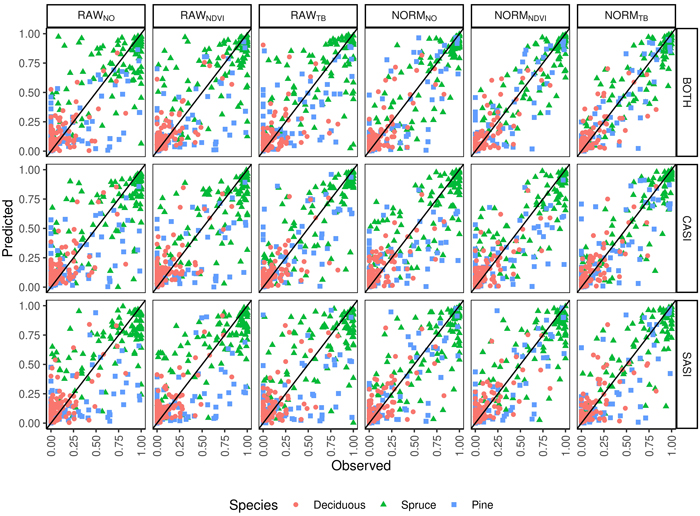
Fig. 4. Observed and predicted species proportions (Spruce = Norway spruce (Picea abies), Pine = Scots pine (Pinus sylvestris), Deciduous (mainly birch (Betula spp.))) for different sensors (CASI, SASI) and their combination (BOTH) for different preprocessing steps (RAWNO, RAWNDVI, RAWTB, NORMNO, NORMNDVI, NORMTB).
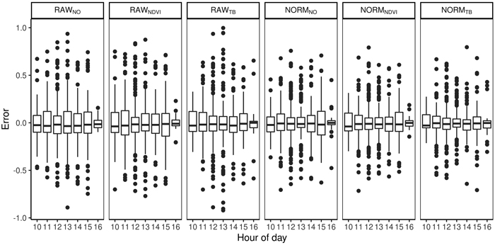
Fig. 5. Difference between predicted and observed species proportions for different hours of the day and for different preprocessing steps (RAWNO, RAWNDVI, RAWTB, NORMNO, NORMNDVI, NORMTB).
| Table 4. Results for species-specific volume and fuzzy set accuracy for the Dirichlet regression approach. OA = overall accuracy, RRMSDS = relative root mean squared error for Norway spruce (Picea abies), RRMSDP = relative root mean squared error for Scots pine (Pinus sylvestris), RRMSDD = relative root mean squared error for deciduous trees (mainly birch (Betula spp.)). | |||||||||||
| Data | Sensor | Kappa-value | OA | RRMSDS | RRMSDP | RRMSDD | Fuzzy set accuracy | ||||
| Five | Four | Three | Two | One | |||||||
| RAWNO | CASI | 0.53 | 0.81 | 48 | 142.3 | 142.6 | 50 | 73 | 85 | 15 | 11 |
| RAWNO | SASI | 0.39 | 0.77 | 42.6 | 150.6 | 139.7 | 45 | 74 | 83 | 18 | 11 |
| RAWNO | BOTH | 0.53 | 0.81 | 46.6 | 139.5 | 128 | 53 | 76 | 85 | 16 | 10 |
| RAWNDVI | CASI | 0.69 | 0.87 | 47.2 | 148.3 | 140.8 | 51 | 75 | 86 | 13 | 8 |
| RAWNDVI | SASI | 0.43 | 0.79 | 41.2 | 148.6 | 134.8 | 47 | 72 | 86 | 14 | 9 |
| RAWNDVI | BOTH | 0.55 | 0.82 | 46.6 | 146.6 | 114.7 | 57 | 76 | 86 | 14 | 10 |
| RAWTB | CASI | 0.61 | 0.84 | 41.2 | 120.2 | 107.5 | 61 | 83 | 90 | 10 | 6 |
| RAWTB | SASI | 0.57 | 0.82 | 48.6 | 146.3 | 154.4 | 48 | 72 | 85 | 15 | 10 |
| RAWTB | BOTH | 0.52 | 0.8 | 48.1 | 134.7 | 123.5 | 57 | 78 | 86 | 14 | 10 |
| NORMNO | CASI | 0.42 | 0.77 | 37.8 | 135.8 | 124.6 | 53 | 73 | 85 | 16 | 8 |
| NORMNO | SASI | 0.66 | 0.86 | 40.6 | 114.2 | 148.9 | 58 | 78 | 87 | 12 | 6 |
| NORMNO | BOTH | 0.66 | 0.85 | 35 | 117.6 | 117.6 | 64 | 81 | 90 | 9 | 5 |
| NORMNDVI | CASI | 0.62 | 0.85 | 35.4 | 131.5 | 129.4 | 60 | 76 | 87 | 13 | 5 |
| NORMNDVI | SASI | 0.65 | 0.86 | 37.7 | 120.6 | 124 | 58 | 81 | 91 | 8 | 5 |
| NORMNDVI | BOTH | 0.79 | 0.91 | 32.4 | 104.9 | 109.6 | 68 | 84 | 93 | 6 | 2 |
| NORMTB | CASI | 0.76 | 0.9 | 36.6 | 105 | 100 | 66 | 85 | 92 | 8 | 4 |
| NORMTB | SASI | 0.69 | 0.87 | 38.1 | 122.9 | 132.3 | 64 | 82 | 92 | 8 | 6 |
| NORMTB | BOTH | 0.70 | 0.88 | 34.2 | 87 | 102.2 | 68 | 88 | 93 | 6 | 2 |
3.2 Dominant species classification
The overall accuracy ranged between 0.77 and 0.91 and kappa-values ranged between 0.39 and 0.79 (Table 4). On average, the CASI sensor produced larger kappa values than the SASI sensor (0.60 vs 0.56) and combining the sensor increased the average kappa slightly (0.62). The producer’s accuracy was always high for spruce (>87%) for all preprocessing alternatives. However, producer’s accuracy of pine-dominated plots are only above 50% in three of the cases using RAW data and contribute to the small accuracies of these preprocessing alternatives. Thus, overall applying the normalization improved the classification performance from an average kappa of 0.53 to 0.66 (Fig. 6). The exception is for the CASI sensor when not applying the TB thresholding. The reason for this is the higher number of misclassification of pine-dominated plots as spruce (Table 5). The misclassification of pine-dominated plots with spruce-dominated plot also explains the large increase in accuracy using normalization on SASI and the combined sensors. Similarly, the average kappa-value applying either NDVI threshold (0.62) or TB threshold (0.64) was higher than NO threshold on average (0.53). The TB threshold had higher accuracies for single CASI, while there was no difference using the SASI sensor and NDVI threshold was higher for the combination of sensors.
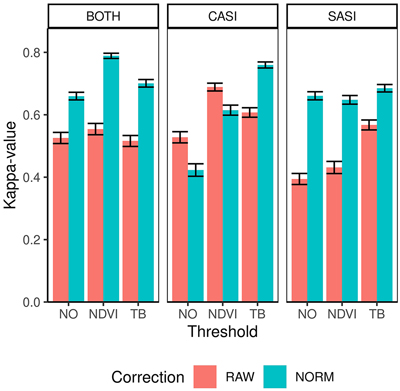
Fig. 6. Kappa values and confidence intervals for dominant species obtained by different sensors (CASI and SASI) and their combination (BOTH). In addition, the different preprocessing steps, i.e., using raw data (RAW) or normalized data (NORM) and different thresholding methods (NO, NDVI or TB).
| Table 5. Error matrices of the dominant species classification (S = Norway spruce (Picea abies), P = Scots pine (Pinus sylvestris), D = deciduous (mainly birch (Betula spp.))) obtained from the Dirichlet regression for different sensors (CASI, SASI and combined BOTH) and preprocessing methods (Data). PA = producer’s accuracy and UA = User’s accuracy. | |||||||||||||
| Data | Sensor | CASI | SASI | BOTH | |||||||||
| Species | S | P | D | PA | S | P | D | PA | S | P | D | PA | |
| RAWNO | S | 65 | 11 | 1 | 84.4 | 66 | 13 | 2 | 81.5 | 65 | 10 | 2 | 84.4 |
| P | 3 | 10 | 0 | 76.9 | 2 | 6 | 0 | 75.0 | 3 | 11 | 0 | 78.6 | |
| D | 2 | 1 | 4 | 57.1 | 2 | 3 | 3 | 37.5 | 2 | 1 | 3 | 50.0 | |
| UA | 92.9 | 45.5 | 80.0 | 81.4 | 94.3 | 27.3 | 60.0 | 77.3 | 92.9 | 50.0 | 60.0 | 81.4 | |
| RAWNDVI | S | 64 | 6 | 0 | 91.4 | 67 | 15 | 1 | 80.7 | 65 | 12 | 0 | 84.4 |
| P | 4 | 15 | 0 | 78.9 | 1 | 6 | 0 | 85.7 | 3 | 10 | 0 | 76.9 | |
| D | 2 | 1 | 5 | 62.5 | 2 | 1 | 4 | 57.1 | 2 | 0 | 5 | 71.4 | |
| UA | 91.4 | 68.2 | 100.0 | 86.6 | 95.7 | 27.3 | 80.0 | 79.4 | 92.9 | 45.5 | 100.0 | 82.5 | |
| RAWTB | S | 63 | 6 | 2 | 88.7 | 65 | 9 | 1 | 86.7 | 63 | 8 | 3 | 85.1 |
| P | 6 | 15 | 0 | 71.4 | 3 | 11 | 0 | 78.6 | 5 | 13 | 0 | 72.2 | |
| D | 1 | 1 | 3 | 60.0 | 2 | 2 | 4 | 50.0 | 2 | 1 | 2 | 40.0 | |
| UA | 90.0 | 68.2 | 60.0 | 83.5 | 92.9 | 50.0 | 80.0 | 82.5 | 90.0 | 59.1 | 40.0 | 80.4 | |
| NORMNO | S | 63 | 13 | 1 | 81.8 | 64 | 5 | 2 | 90.1 | 61 | 4 | 1 | 92.4 |
| P | 5 | 8 | 0 | 61.5 | 2 | 16 | 0 | 88.9 | 4 | 17 | 0 | 81.0 | |
| D | 2 | 1 | 4 | 57.1 | 4 | 1 | 3 | 37.5 | 5 | 1 | 4 | 40.0 | |
| UA | 90.0 | 36.4 | 80.0 | 77.3 | 91.4 | 72.7 | 60.0 | 85.6 | 87.1 | 77.3 | 80.0 | 84.5 | |
| NORMNDVI | S | 65 | 9 | 1 | 86.7 | 65 | 5 | 3 | 89.0 | 66 | 3 | 0 | 95.7 |
| P | 3 | 13 | 0 | 81.2 | 3 | 16 | 0 | 84.2 | 1 | 17 | 0 | 94.4 | |
| D | 2 | 0 | 4 | 66.7 | 2 | 1 | 2 | 40.0 | 3 | 2 | 5 | 50.0 | |
| UA | 92.9 | 59.1 | 80.0 | 84.5 | 92.9 | 72.7 | 40.0 | 85.6 | 94.3 | 77.3 | 100.0 | 90.7 | |
| NORMTB | S | 66 | 3 | 1 | 94.3 | 65 | 4 | 2 | 91.5 | 66 | 5 | 2 | 90.4 |
| P | 3 | 17 | 0 | 85.0 | 2 | 16 | 0 | 88.9 | 1 | 16 | 0 | 94.1 | |
| D | 1 | 2 | 4 | 57.1 | 3 | 2 | 3 | 37.5 | 3 | 1 | 3 | 42.9 | |
| UA | 94.3 | 77.3 | 80.0 | 89.7 | 92.9 | 72.7 | 60.0 | 86.6 | 94.3 | 72.7 | 60.0 | 87.6 | |
3.3 Species-specific volume
The RMSD obtained for the different species range from 55.5–81.8 m3 ha–1 (32.4–48.6%) for spruce, 41.6–72.0 m3 ha–1 (87.0–150.6%) for pine and 25.4 to 39.3 m3 ha–1 (100.0–154.4%) for deciduous species (Table 4). On average, the accuracy was better for CASI than SASI and the combination made additional improvements. However, the differences between the sensors were most prominent for pine and deciduous species, with a decrease of 12 and 23 percentage points in RRMSD, respectively, using only SASI or the sensor combination (Fig. 7). The differences for spruce was negligible (1 percentage point). Overall the normalization provided lower RRMSDs than using the raw data. The improvements were 9.1, 26.4 and 10.8 percentage points for spruce, pine and deciduous species, respectively. The choice of threshold had only minor improvements on spruce volume. On average, the TB threshold improved the accuracy of pine and deciduous species, while the NDVI threshold only improved deciduous volume.
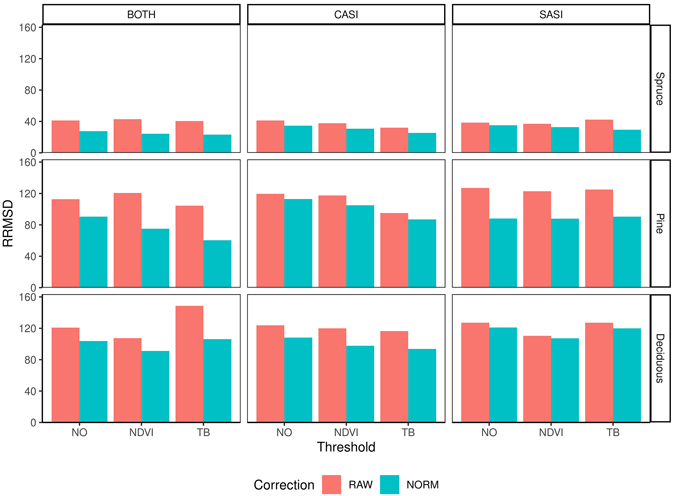
Fig. 7. Relative root mean square difference (RRMSD) for different preprocessing steps, i.e., using raw data (RAW) or normalized data (NORM), and thresholding methods (NO, NDVI, TB), species (Spruce = Norway spruce (Picea abies), Pine = Scots pine (Pinus sylvestris), Deciduous (mainly birch (Betula spp.))), sensors (CASI and SASI) and their combination (BOTH).
3.4 Species proportions as tenths
The accuracy of the tenths as measured by the Score values range from 48.1–70.1% for plots deviation less than 10% (Score 5) and 82.8–93.8% as plots with a deviation of less than 30% (Score 3) (Table 4, Fig. 8. On average, there are small differences between the sensors, but the combination of sensors produces the best results. Furthermore, on average the normalization increased the proportion of plots in score values 5, 4, 3 by 10.0, 5.3 and 4.5 percentage points. The normalization improves the score values for spruce and pine using the SASI sensor or the combined sensors. When applying the CASI sensor improvements are mainly connected to the improvement of the most accurate plots (Score 5). Similarly, applying either NDVI or TB threshold improved the Score values by 7.2, 6.0, 3.7 for TB thresholding and 3.2, 1.9 and 2.4 for NDVI thresholding. Particularly, the improvement is for score 5 for deciduous species for both sensors. For spruce, the improvement is in the most accurate plots (Score 5) for the CASI sensor. Furthermore, the normalization improves all score values of pine and spruce when using SASI.
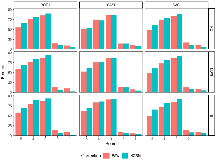
Fig. 8. Percentage of observations in different score values (5–1) obtained from fuzzy validation by different sensors (CASI and SASI) and their combination (BOTH). In addition, the different preprocessing steps, i.e., using raw data (RAW) or normalized data (NORM) and different thresholding methods (NO, NDVI or TB). A score of 5 indicates no deviation between predicted and observed species proportion and a lower score indicates subsequent higher deviation; for details see section 2.4.3.
3.5 Important wavelengths
The selected variables for the different datasets were analyzed to guide the selection of other hyperspectral sensors to be used in FMIs in the boreal forests (objective 3). For the datasets without normalization, the most frequently selected variables were located in the red edge (673–730 nm) and infrared (950–1300 and 1662–1677 nm) parts of the spectrum (Fig. 9). For the normalized datasets, the computed indices were frequently selected together with variables from the ultraviolet (368–378 nm), the edge between green and blue (490 nm), the red edge (692 nm), and the infrared (950–1050 and 1662 nm) parts of the spectrum.
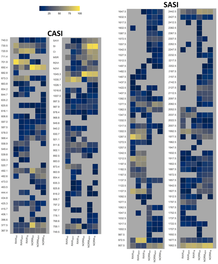
Fig. 9. Relative importance of HS-derived variables, i.e., vegetation index name or wavelength obtained by different sensors (CASI and SASI) and the different preprocessing steps, i.e., using raw data (RAW) or normalized data (NORM) and different thresholding methods (NO, NDVI or TB). Importance was computed as the percentage the variable was selected in the cross-validation. View larger in new window/tab.
4 Discussion
4.1 Area-based methodology for hyperspectral data
A limitation of the Dirichlet regression is that small proportions are overestimated and that large proportions are underestimated. Furthermore, the small proportions of deciduous trees occurring in the Scandinavian boreal forests also limit the accuracy obtained for these species. In our study, there are only five sample plots dominated by deciduous species. Although we evaluate dominant species in terms of the kappa coefficient, this is a limitation of the study. Accurate identification of minority species likely requires other methods or sampling procedures. For species-specific information in FMIs the information about the most valuable species i.e., spruce and pine is of higher priority. Irrespective of limitations, we find the Dirichlet regression a suitable method for predicting species proportions and deriving dominant species, species-specific volumes in the boreal forest following an area-based methodology.
Hyperspectral data were normalized following conventional methods by scaling the band pixel value relative to the sum of all band values within the pixel. Three different methods for thresholding were evaluated in combination with the normalization. Normalization showed, in general, a positive effect on the different evaluation criteria using hyperspectral data, mainly by improving predictions of spruce and pine. Furthermore, the results improved by applying the novel TB thresholding, especially using data from the CASI sensor or SASI sensor separately. The combination of normalization and TB thresholding resulted in the smallest errors overall. However, NDVI thresholding produced almost similar results as the TB thresholding for the SASI and combined sensors. Thus, both normalization and thresholding are recommended.
The results using data from the two sensors did not differ much. Although the CASI sensor resulted in the largest accuracy overall, it seems that both CASI and SASI could capture the information used to separate species. Combining the sensors slightly improved the accuracies in most cases.
The analysis of the variables selected for modeling the species composition gives us an insight into the importance of different wavelength regions. For the RAW datasets and without normalization, the variables which were most frequently selected to be included in the models were located in the red edge (670–760 nm), the near-infrared (950–1300 nm), and short-wave infrared (1660 and 2000 nm) parts of the spectrum. For the normalized datasets, selected variables were found in the same spectral range as the RAW datasets. However, very few variables were selected in the range from 1100 nm to 1300 nm compared to the RAW datasets. Furthermore, computed indices were more frequently selected from the normalized data. The importance of the red-edge region is found in other boreal studies (Heikkinen et al. 2010; Pant et al. 2013, 2014). Fassnacht et al. (2016) reviewed results from 13 studies based on hyperspectral data and found that the most important wavelength regions were 450–550 nm, 650–700 nm, 1150–1200 nm, 1450 nm, and 2000 nm. Our results confirm the importance of data from many of these wavelength regions, but differences also exist, as one might expect in individual studies. Primarily 450–550 nm are important in other boreal studies (Heikkinen et al. 2010; Pant et al. 2014), but not in the current study.
4.2 Comparison of obtained accuracy
The accuracy at plot level obtained using the ALS data (RRMSD = 23%) is similar to what is found in previous studies (Næsset 2002). The accuracy could probably have been improved using stratum-specific models, which were not used in the current study. Furthermore, sample plots with a large proportion of deciduous species are commonly excluded from ALS-based FMIs in Norway. In the current study, these plots were included and this may have influenced the final accuracy. However, a stratification and an exclusion of deciduous plots would conflict with the aim of the current study; species composition is important both for stratification and for identifying areas with large proportions of deciduous species. Mitigating the unbalances in species composition in an inventory area by changing the allocation of sample plots to improve species-specific inventories are suggested for non-parametric methods (Vauhkonen et al. 2012; Räty et al. 2016) and partly achieved with stratification for parametric methods (Næsset 2002). Thus, there is a need to investigate sampling frameworks accounting for such imbalances for parametric methods.
Results of species-specific volume modeling are often evaluated in terms of RMSD. Puliti et al. (2017a) reported RMSD and RRMSD of 72 m3 ha–1, 45 m3 ha–1, 35 m3 ha–1 and 49%, 63%, and 114%, respectively for spruce, pine and deciduous species obtained using photogrammetric point cloud data in Norway. Furthermore, using a combination of multispectral imagery and ALS (Maltamo et al. 2015) reported RRMSD of 30%, 55%, and 122% for the species-specific volumes of the tree species. In the current study, RMSD values of 58 m3 ha–1, 42 m3 ha–1, 26 m3 ha–1 and RRMSD values of 34%, 87%, and 102% were obtained for spruce, pine and deciduous species. Comparing the results of species-specific volumes between different studies in terms of RMSD is challenging because the basis for comparison differs with regard to the size of the reference unit, i.e., species-specific average volume and average total volume. The small volumes of pine and deciduous species compared to spruce (Table 2) result in smaller RRMSD values for spruce and larger values for pine and deciduous.
The accuracy obtained for the dominant species is often reported in studies concerning species composition. In boreal forests, Maltamo et al. (2015) reported results for the dominant species obtained by photo-interpretation on 80 field plots of size 1000 m2 and compared to prediction using ALS and aerial multispectral images. The study reported a kappa-value of 0.59 and OA of 83% for the photo-interpretation and 0.89 and 95% for the prediction using remotely sensed data (Maltamo et al. 2015). Using the area-based approach and ALS data combined with hyperspectral data in the boreal forest a kappa-value of 0.91 and overall accuracy of 96% were obtained (Ørka et al. 2013). In the current study, the largest kappa-value and OA were 0.79 and 91%, respectively.
Fuzzy set validation is reported in relatively few studies. The method was used to assess species proportions obtained by manual photo-interpretation (Magnusson et al. 2007). However, in many forest management plans, species information is provided in terms of species proportions rounded to tenths. Thus, from a practical point of view, this is an meaningful comparison. The scores obtained by Magnusson et al. (2007) from score five to one were 48, 84, 96, 4, 2 and 33, 79, 94, 6, 2 for two different base ratios on average of four interpreters. Using ALS data and hyperspectral data in combination, Ørka et al. (2013) obtained score values of 30, 86, 96, 4, 0(from score five to one) using the non-parametric random forest algorithm for prediction. However, both these studies used larger units for their field reference than in the current study, i.e., forest stands with an average size of 3 ha (Magnusson et al. 2007) and field plots of 1000 m2 (Ørka et al. 2013), respectively. Thus, our results from the fuzzy set evaluation with score values of 68, 88, 93, 6, 2, (from score five to one) seem reasonable in this comparison. We have a slightly smaller cumulative percentage of score 3 ‘‘acceptable answer’’ (deviation of two-tenths) than both the above-mentioned studies. Nevertheless, the score 5 ‘‘absolutely right’’ (no deviation between field measurements of tree species) was larger. Taking into account the small area covered by a “grid-cell” we consider this to be a very good result, especially when considering the variation between interpreters. For score 5 this was 18–61 and for score 3 it ranged between 89–100 for the interpreters in the study by Magnusson et al. (2007).
4.3 Costs and operationalizing
At the moment (2021), the acquisition of hyperspectral data costs around 2.5 EUR ha–1 (1.0–3.5 EUR ha–1) in Norway, while the cost of acquiring ordinary aerial photographs and carrying out manual photo-interpretation is about 5.5 EUR ha–1 (Eid et al. 2004). The costs of ALS and hyperspectral data have decreased substantially in recent years. In contrast, the hourly wages for manual photo-interpretation have increased, but due to the reuse of older management plans and thus reduced interpretation time, the total photo-interpretation cost has been more or less constant. The current research indicates that accuracies similar to those of photo-interpretation can be obtained using hyperspectral data, thus, indicating similar losses due to erroneous data. However, it would be beneficial to carry out a cost-plus-loss analysis (Eid et al. 2004) comparing the conventional two-step procedure based on ALS data and manual photo-interpretation, with a procedure using ALS data and automated hyperspectral classification and delineation. This would be useful to guide future decisions on inventory methodology for operational FMIs.
5 Conclusions
The current study combines airborne laser scanning and hyperspectral data in a two-stage procedure to provide species information in boreal forests. Using the Dirichlet regression provides consistent estimates of species proportions, species-specific volume and dominant species. The approach produced acceptable results in approximately 90% of the plots (i.e., less than or 30% deviation). The normalization and a tree-based selection of pixels provided the best results, although selecting pixels based on NDVI also yielded good results. The visible to near-infrared sensor gave overall better results. However the near to shortwave-infrared also provided good results. The combined use of the two sensors produced slightly better results than using either of them separately. The important wavelength regions identified varied among the different normalization and thresholding methods, but our results align with the current literature.
Authors’ contributions
Hans Ole Ørka: Conceptualization, Methodology, Formal analysis, Investigation, Writing - Original Draft, Writing - Review & Editing, Visualization, Project administration, Funding acquisition, Final approval. Endre Hofstad Hansen: Conceptualization, Methodology,Formal analysis, Writing - Original Draft, Writing - Review & Editing, Visualization, Final approval. Michele Dalponte: Conceptualization, Methodology, Formal analysis, Investigation,Writing - review & editing, Final approval. Terje Gobakken: Conceptualization, Methodology, Writing - Review & Editing, Project administration, Funding acquisition, Final approval. Erik Næsset: Conceptualization, Methodology, Writing - Review & Editing, Funding acquisition, Final approval.
Funding
This research was conducted as a part of the HyperBio project supported by BIONÆR program of the Research Council of Norway and TerraTec AS (grant no. 244599).
Acknowledgments
We would like to thank the field crews from Mjøsen Skog SA, TerraTec AS, and Norwegian University of Life Sciences, Faculty of Environmental Sciences and Natural Resource Management, who helped collect the field data. Furthermore, we also want to thank Terratec for the collection and preprocessing of the remotely sensed data. Lastly, we want to thank two anonymous reviewers for providing constructive comments on an earlier version of the manuscript.
References
Avery TE, Burkhart HE (2015) Forest measurements. Waveland Press, Long Grove, IL.
Braastad H (1966) Volume tables for birch. Reports of the Norwegian Forest Research Institute 21: 265–365.
Brantseg A (1967) Volume functions and tables for Scots pine. South Norway. Reports of the Norwegian Forest Research Institute 12: 689–739.
Chen JM (1996) Evaluation of vegetation indices and a modified simple ratio for boreal applications. Can J Remote Sens 22: 229–242. https://doi.org/10.1080/07038992.1996.10855178.
Coomes DA, Dalponte M, Jucker T, Asner GP, Banin LF, Burslem DFRP, Lewis SL, Nilus R, Phillips OL, Phua M-H, Qie L (2017) Area-based vs tree-centric approaches to mapping forest carbon in Southeast Asian forests from airborne laser scanning data. Remote Sens Environ 194: 77–88. https://doi.org/10.1016/j.rse.2017.03.017.
Dalponte M, Ørka HO, Gobakken T, Gianelle D, Næsset E (2013) Tree species classification in boreal forests with hyperspectral data. IEEE Trans Geosci Remote Sens 51: 2632–2645. https://doi.org/10.1109/TGRS.2012.2216272.
Dalponte M, Ørka HO, Ene LT, Gobakken T, Næsset E (2014) Tree crown delineation and tree species classification in boreal forests using hyperspectral and ALS data. Remote Sens Environ 140: 306–317. https://doi.org/10.1016/j.rse.2013.09.006.
Dalponte M, Reyes F, Kandare K, Gianelle D (2015) Delineation of individual tree crowns from ALS and hyperspectral data: a comparison among four methods. Eur J Remote Sens 48: 365–382. https://doi.org/10.5721/EuJRS20154821.
Dalponte M, Frizzera L, Ørka HO, Gobakken T, Næsset E, Gianelle D (2018) Predicting stem diameters and aboveground biomass of individual trees using remote sensing data. Ecol Indic 85: 367–376. https://doi.org/10.1016/j.ecolind.2017.10.066.
Donoghue D, Watt P, Cox N, Wilson J (2007) Remote sensing of species mixtures in conifer plantations using LiDAR height and intensity data. Remote Sens Environ 110: 509–522. https://doi.org/10.1016/j.rse.2007.02.032.
Eid T, Gobakken T, Næsset E (2004) Comparing stand inventories for large areas based on photo-interpretation and laser scanning by means of cost-plus-loss analyses. Scand J For Res 19: 512–523. https://doi.org/10.1080/02827580410019463.
Fassnacht FE, Latifi H, Stereńczak K, Modzelewska A, Lefsky M, Waser LT, Straub C, Ghosh A (2016) Review of studies on tree species classification from remotely sensed data. Remote Sens Environ 186: 64–87. https://doi.org/10.1016/j.rse.2016.08.013.
Fitje A, Vestjordet E (1977) Stand height curves and new tariff tables for Norway spruce. Norwegian Forest Research Institute, Ås.
Gao T, Hedblom M, Emilsson T, Nielsen AB (2014) The role of forest stand structure as biodiversity indicator. For Ecol Manage 330: 82–93. https://doi.org/10.1016/j.foreco.2014.07.007.
Gopal S, Woodcock C (1994) Theory and methods for accuracy assessment of thematic maps using fuzzy sets. Photogramm Eng Remote Sens 60: 181–188.
Haara A, Kangas A, Tuominen S (2019) Economic losses caused by tree species proportions and site type errors in forest management planning. Silva Fenn 53, article id 10089. https://doi.org/10.14214/sf.10089.
Haboudane D, Miller JR, Pattey E, Zarco-Tejada PJ, Strachan IB (2004) Hyperspectral vegetation indices and novel algorithms for predicting green LAI of crop canopies: modeling and validation in the context of precision agriculture. Remote Sens Environ 90: 337–352. https://doi.org/10.1016/j.rse.2003.12.013.
Heikkinen V, Tokola T, Parkkinen J, Korpela I, Jaaskelainen T (2010) Simulated multispectral imagery for tree species classification using support vector machines. IEEE Trans Geosci Remote Sens 48: 1355–1364. https://doi.org/10.1109/TGRS.2009.2032239.
Hijazi RH, Jernigan RW (2009) Modelling compositional data using Dirichlet regression models. J Appl Probab Stat 4: 77–91.
Holmgren J, Persson Å, Söderman U (2008) Species identification of individual trees by combining high resolution LiDAR data with multi‐spectral images. Int J Remote Sens 29: 1537–1552. https://doi.org/10.1080/01431160701736471.
Hovi A, Raitio P, Rautiainen M (2017) A spectral analysis of 25 boreal tree species. Silva Fenn 51, article id 7753 https://doi.org/10.14214/sf.7753.
Huete AR (1988) A soil-adjusted vegetation index (SAVI). Remote Sens Environ 25: 295–309. https://doi.org/10.1016/0034-4257(88)90106-X.
Kandare K, Dalponte M, Ørka HO, Frizzera L, Næsset E (2017a) Prediction of species-specific volume using different inventory approaches by fusing airborne laser scanning and hyperspectral data. Remote Sensing 9, article id 400. https://doi.org/10.3390/rs9050400.
Kandare K, Ørka HO, Dalponte M, Næsset E, Gobakken T (2017b) Individual tree crown approach for predicting site index in boreal forests using airborne laser scanning and hyperspectral data. Int J Appl Earth Obs Geoinf 60: 72–82. https://doi.org/10.1016/j.jag.2017.04.008.
Kim S, Sohn K-A, Xing EP (2009) A multivariate regression approach to association analysis of a quantitative trait network. Bioinformatics 25: i204–i212. https://doi.org/10.1093/bioinformatics/btp218.
Kovac M, Gasparini P, Notarangelo M, Rizzo M, Cañellas I, Fernández-de-Uña L, Alberdi I (2020) Towards a set of national forest inventory indicators to be used for assessing the conservation status of the habitats directive forest habitat types. J Nat Conserv 53, article id 125747. https://doi.org/10.1016/j.jnc.2019.125747.
Lima F (2018) GFLASSO: Graph-Guided Fused LASSO in R. https://www.datacamp.com/community/tutorials/gflasso-R. Accessed 2 Nov 2020.
Lumley T, Miller A (2009) Leaps: regression subset selection, R package version 2.
Magnusson M, Fransson JES, Olsson H (2007) Aerial photo-interpretation using Z/I DMC images for estimation of forest variables. Scand J For Res 22: 254–266. https://doi.org/10.1080/02827580701262964.
Maier MJ (2014) DirichletReg: Dirichlet regression for compositional data in R. Institute for Statistics and Mathematics Report.
Maltamo M, Packalen P (2014) Species-specific management inventory in Finland. In: Maltamo M, Næsset E, Vauhkonen J (eds) Forestry applications of airborne laser scanning. Springer Netherlands, pp 241–252. https://doi.org/10.1007/978-94-017-8663-8_12.
Maltamo M, Ørka HO, Bollandsås OM, Gobakken T, Næsset E (2015) Using pre-classification to improve the accuracy of species-specific forest attribute estimates from airborne laser scanner data and aerial images. Scand J For Res 30: 336–345. https://doi.org/10.1080/02827581.2014.986520.
Mora B, Wulder MA, White JC (2010) Identifying leading species using tree crown metrics derived from very high spatial resolution imagery in a boreal forest environment. Can J Remote Sens 36: 332–344. https://doi.org/10.5589/m10-052.
Morais J, Thomas-Agnan C, Simioni M (2017) Using compositional and Dirichlet models for market share regression. J Appl Stat 1–20. https://doi.org/10.1080/02664763.2017.1389864.
Næsset E (2002) Predicting forest stand characteristics with airborne scanning laser using a practical two-stage procedure and field data. Remote Sens Environ 80: 88–99. https://doi.org/10.1016/S0034-4257(01)00290-5.
Næsset E (2014) Area-based inventory in Norway – from innovation to an operational reality. In: Maltamo M, Næsset E, Vauhkonen J (eds) Forestry applications of airborne laser scanning. Springer, pp 215–240. https://doi.org/10.1007/978-94-017-8663-8_11.
Næsset E, Gobakken T (2008) Estimation of above- and below-ground biomass across regions of the boreal forest zone using airborne laser. Remote Sens Environ 112: 3079–3090. https://doi.org/10.1016/j.rse.2008.03.004.
Ørka HO, Gobakken T, Næsset E, Ene L, Lien V (2012) Simultaneously acquired airborne laser scanning and multispectral imagery for individual tree species identification. Can J Remote Sens 38: 125–138. https://doi.org/10.5589/m12-021.
Ørka HO, Dalponte M, Gobakken T, Næsset E, Ene LT (2013) Characterizing forest species composition using multiple remote sensing data sources and inventory approaches. Scand J For Res 28: 677–688. https://doi.org/10.1080/02827581.2013.793386.
Otsu N (1979) A threshold selection method from gray-level histograms. Automatica 11: 23–27.
Packalén P, Maltamo M (2008) Estimation of species-specific diameter distributions using airborne laser scanning and aerial photographs. Can J Forest Res 38: 1750–1760. https://doi.org/10.1139/x08-037.
Packalén P, Suvanto A, Maltamo M (2009) A two stage method to estimate species-specific growing stock. Photogramm Eng Remote Sens 75: 1451–1460. https://doi.org/10.14358/PERS.75.12.1451.
Pant P, Heikkinen V, Hovi A, Korpela I, Hauta-Kasari M, Tokola T (2013) Evaluation of simulated bands in airborne optical sensors for tree species identification. Remote Sens Environ 138: 27–37. https://doi.org/10.1016/j.rse.2013.07.016.
Pant P, Heikkinen V, Korpela I, Hauta-Kasari M, Tokola T (2014) Logistic regression-based spectral band selection for tree species classification: effects of spatial scale and balance in training samples. IEEE Geosci Remote S 11: 1604–1608. https://doi.org/10.1109/LGRS.2014.2301864.
Persson Å, Holmgren J, Söderman U (2002) Detecting and measuring individual trees using an airborne laser scanner. Photogramm Eng Remote Sens 68: 925–932.
Peuhkurinen J, Maltamo M, Malinen J (2008) Estimating species-specific diameter distributions and saw log recoveries of boreal forests from airborne laser scanning data and aerial photographs: a distribution-based approach. Silva Fenn 42: 625–641. https://doi.org/10.14214/sf.237.
Puliti S, Gobakken T, Ørka HO, Næsset E (2017a) Assessing 3D point clouds from aerial photographs for species-specific forest inventories. Scand J For Res 32: 68–79. https://doi.org/10.1080/02827581.2016.1186727.
Puliti S, Ene LT, Gobakken T, Næsset E (2017b) Use of partial-coverage UAV data in sampling for large scale forest inventories. Remote Sens Environ 194: 115–126. https://doi.org/10.1016/j.rse.2017.03.019.
R Core Team (2019) R: a language and environment for statistical computing, version 3.5.3. R Foundation for Statistical Computing, Vienna, Austria. https://www.R-project.org/.
Räty J, Vauhkonen J, Maltamo M, Tokola T (2016) On the potential to predetermine dominant tree species based on sparse-density airborne laser scanning data for improving subsequent predictions of species-specific timber volumes. For Ecosyst 3, article id 1. https://doi.org/10.1186/s40663-016-0060-0.
Roujean J-L, Breon F-M (1995) Estimating PAR absorbed by vegetation from bidirectional reflectance measurements. Remote Sens Environ 51: 375–384. https://doi.org/10.1016/0034-4257(94)00114-3.
Rouse JW, Haas RH, Schell JA, Deering DW, Harlan JC (1973) Monitoring the vernal advancement and retrogradation of natural vegetation [NASA/GSFCT Type II Report]. NASA/Goddard Space Flight Center, Greenbelt, MD.
Sankaran K, De Abreu e Lima F (2018) gflasso: perform graph structured multitask regression, version 0.0.0.9000. https://github.com/krisrs1128/gflasso.
Soininen A (2016) TerraScan User’s Guide.
Trier ØD, Salberg A-B, Kermit M, Rudjord Ø, Gobakken T, Næsset E, Aarsten D (2018) Tree species classification in Norway from airborne hyperspectral and airborne laser scanning data. Eur J Remote Sens 51: 336–351. https://doi.org/10.1080/22797254.2018.1434424.
Vaglio Laurin G, Puletti N, Hawthorne W, Liesenberg V, Corona P, Papale D, Chen Q, Valentini R (2016) Discrimination of tropical forest types, dominant species, and mapping of functional guilds by hyperspectral and simulated multispectral Sentinel-2 data. Remote Sens Environ 176: 163–176. https://doi.org/10.1016/j.rse.2016.01.017.
Vauhkonen J, Seppänen A, Packalén P, Tokola T (2012) Improving species-specific plot volume estimates based on airborne laser scanning and image data using alpha shape metrics and balanced field data. Remote Sens Environ 124: 534–541. https://doi.org/10.1016/j.rse.2012.06.002.
Vestjordet E (1967) Functions and tables for volume of standing trees. Norway spruce. Reports of the Norwegian Forest Research Institute 22: 539–574.
Vihervaara P, Mononen L, Auvinen A-P, Virkkala R, Lü Y, Pippuri I, Packalen P, Valbuena R, Valkama J (2015) How to integrate remotely sensed data and biodiversity for ecosystem assessments at landscape scale. Landsc Ecol 30: 501–516. https://doi.org/10.1007/s10980-014-0137-5.
Yu B, Ostland M, Gong P, Pu R (1999) Penalized discriminant analysis of in situ hyperspectral data for conifer species recognition. IEEE Trans Geosci Remote Sens 37: 2569–2577. https://doi.org/10.1109/36.789651.
Total of 60 references.
