Tomi Karjalainen  ,
Petteri Packalen,
Janne Räty,
Matti Maltamo
,
Petteri Packalen,
Janne Räty,
Matti Maltamo
Predicting factual sawlog volumes in Scots pine dominated forests using airborne laser scanning data
Karjalainen T., Packalen P., Räty J., Maltamo M. (2019). Predicting factual sawlog volumes in Scots pine dominated forests using airborne laser scanning data. Silva Fennica vol. 53 no. 4 article id 10183. https://doi.org/10.14214/sf.10183
Highlights
- We predicted visually bucked factual sawlog volumes at the 30 × 30 m plot-level with several alternatives
- The lowest root mean squared error value of approximately 21% was obtained with a linear mixed-effects model that employed factual sawlog volume as a response variable and airborne laser scanning metrics as predictors
- The sawlog reduction model commonly used in Finland performed poorly.
Abstract
The aim in the study was to compare alternatives for the prediction of factual sawlog volumes using airborne laser scanning (ALS) data in Scots pine (Pinus sylvestris L.) dominated forests in eastern Finland. Accurate estimates of factual sawlog volume are desirable to ease the planning of harvesting operations. The factual sawlog volume of pines was derived from visual bucking, i.e. a procedure where the defects were located on each stem during sample plot measurements. For other species, the theoretical sawlog volume was considered also as the factual sawlog volume due to data restrictions. We predicted factual sawlog volume with eight alternatives that were based on either linear mixed-effects models or k-nearest neighbour imputations. An existing sawlog reduction model, commonly used in Finland, was also tested individually and combined with a number of the alternatives, and site type information was also utilised. Model fitting and prediction was implemented at the 15 × 15 m level, but accuracy was assessed at the 30 × 30 m level. The relative root mean squared error (RMSE%) values for the factual sawlog volume predictions varied between 20.9% and 33.5%, and the best accuracy was obtained with a linear mixed-effects model. These results indicate that factual sawlog volumes in Scots pine dominated forests can be predicted with reasonable accuracy with ALS data.
Keywords
Pinus sylvestris;
area based approach;
k-NN;
sawlog
-
Karjalainen,
University of Eastern Finland, School of Forest Sciences, P.O. Box 111, FI-80101 Joensuu, Finland
E-mail
tomikar@uef.fi
- Packalen, University of Eastern Finland, School of Forest Sciences, P.O. Box 111, FI-80101 Joensuu, Finland E-mail petteri.packalen@uef.fi
- Räty, University of Eastern Finland, School of Forest Sciences, P.O. Box 111, FI-80101 Joensuu, Finland E-mail janne.raty@uef.fi
- Maltamo, University of Eastern Finland, School of Forest Sciences, P.O. Box 111, FI-80101 Joensuu, Finland E-mail matti.maltamo@uef.fi
Received 25 April 2019 Accepted 6 November 2019 Published 21 November 2019
Views 73702
Available at https://doi.org/10.14214/sf.10183 | Download PDF

1 Introduction
1.1 Background
Airborne laser scanning (ALS) based information has been used in numerous studies to estimate forest characteristics, such as total tree volume and aboveground biomass (Næsset 1997; Næsset 2011). However, the size distribution and quality characteristics of the growing stock are often also needed, especially in harvest planning. The distribution of timber assortments provides essential information, especially from an economic point of view. For example, the value of sawlog in Finland is usually 3–4 times greater than the value of pulpwood.
Sawlog and pulpwood recovery can be estimated by ALS based diameter and height distributions applying taper curves (Peuhkurinen et al. 2008), but this approach does not provide qualitative information about the trees. However, in many cases, qualitative factors such as thick branches, decay and curves in the tree cause sawlog recovery to be considerably smaller than theoretical sawlog recovery might imply. All in all, the prediction of the total value of growing stock prior to harvesting is highly susceptible to errors.
The reduction in factual sawlog volume due to defects can be considered with different sawlog reduction models (Mehtätalo 2002). However, these models usually employ variables that have a tenuous relationship with tree quality (e.g. age, location). Moreover, as they have been fitted from large datasets, the performance on a single stand can be poor. This kind of information is usually adequate for forest planning on large areas (Mehtätalo 2002; Malinen et al. 2007), but knowledge of wood quality in the stand to be harvested is important in the planning of harvest operations. Thus, wood quality data would increase the overall value of forest resource information. The relationship between ALS and wood quality has already been studied to some extent, but there are some fundamental issues that are difficult to overcome. For example, the quality criteria (e.g. minimum diameter and maximum allowed branch thickness) for sawlogs may differ in a case by case basis, meaning that “quality” is difficult to define unambiguously.
1.2 Acquisition of factual sawlog volume data
The main reason for the paucity of research in regard to factual sawlog volumes is that collection of field data is a complicated and laborious task. For the study of factual sawlog volumes, i.e. the effects of different defects are considered, there are essentially only two avenues open for the collection of data. The first option is to use the stem data (stm-file) collected by the harvester (StanForD 2012). This file includes the taper curves of the harvested stems, and so also reveals the rates of sawlog and pulpwood recovery. However, the Cut-To-Length method applied in Finland, for example, produces logs that are already cut in optimal lengths in the felling phase. This means that sawmills have their own preferences for sawlog lengths (and diameters), e.g. minimum length can be 3.7 m and the next approved length is 4.0 m. In such a case, the final 20 cm from a 3.9 m long sawlog would end up in the next pulpwood-log even though it would otherwise fulfil the requirements for a sawlog. At the stand-level, uncertainty accrues from a range of factors that include, for example, the professional ability of the operator (e.g. the operator decides how the defective stems will be cut), the number of retention trees, variation in stump heights (Korhonen et al. 2008) and the mismatch in areas between harvester data and other datasets. The lack of accurate position of a felling head (Holmgren et al. 2012; Lindroos et al. 2015) is also an issue that, to date, has prevented examination of harvester data at the plot- or tree-level. However, e.g. Hauglin et al. (2018) recently used tree-level positioned harvester data to predict volume by ALS. The obtained accuracy level was comparable to field plot-based ground truthing.
The second option to gather factual sawlog volumes is visual bucking of the standing stock, where all the defects that affect the sawlog-proportion of the trunk are detected and recorded during the field measurements. The factual tree-level sawlog volumes are then calculated with stem taper curve models for the parts that fulfil the quality requirements. For instance, this means that the crookedness of the stem for each tree must be evaluated whether it is within the acceptable limits or not, the height of the first excessively thick branch must be measured (assuming the stem diameter is still large enough), and so on. Visual bucking is always a laborious and time-consuming procedure, and should not be used in cases where the defects are mostly internal. However, with Scots pine (Pinus sylvestris L.) the visual bucking is a feasible method as most of the defects are external. The approach is also used in the Finnish National Forest Inventory (Metsäntutkimuslaitos 2009).
1.3 Tree quality in previous studies
In earlier studies, tree quality was mostly studied by predicting factual sawlog volumes. In Finland, Korhonen et al. (2008) used low point density ALS data and built mixed effect regression models to predict factual sawlog volumes at the stand-level. Instead of field determined factual sawlog volumes, they used sawlog reduction model-based estimates in the modelling. The models were tested with harvester data from 14 clear-cut stands. The resulting relative root mean squared error (RMSE%) value for factual sawlog volumes was 18%. The same ALS and harvester data were also used by Peuhkurinen et al. (2008), who first predicted the stand-level height-diameter distributions using ALS (and/or aerial photographs) and the k-Nearest Neighbour (k-NN) method. These predictions were then used to find the nearest neighbouring stands from a separate stem data bank (expanded from the original harvester data), and the final species-specific sawlog recoveries were then estimated based on these neighbouring stem data bank stands. The RMSE% value of the ALS-based sawlog volume was 61.9% for pine and 32.1% for Norway spruce (Picea abies [L.] H. Karst.). These results were not considered satisfactory. In Norway, Bollandsås et al. (2011) used low point density ALS and harvester-based data to create nonlinear mixed-effects models for several quality associated characteristics. Due to restrictions with the accuracy of positioning, the examination was made using grid cells with a size of 50 × 50 m. The prediction of total sawlog volumes resulted in a RMSE% value of 24%. In addition, the individual tree detection (ITD) approach has been used in a number of studies to predict factual sawlog volumes (Peuhkurinen et al. 2007; Maltamo et al. 2009; Barth et al. 2015). In general, the results of these ITD studies have been promising.
1.4 The effect of site fertility on pine quality
It is commonly known that the commercial quality of Scots pine is prone to be worse on fertile sites than on moderate or poor sites. For example, on fertile sites Scots pines often have thick branches also in the lower part of the main stem, and the stems are more often crooked (Lämsä et al. 1990). If strict requirements for sawlogs are applied, these properties may completely prevent the bucking of sawlogs. In Finland, site fertility is described with categorical site type index system presented by Cajander (1949). Site type index can easily be determined for each plot during field measurements and this information is existing all over the country. Therefore, it can also be utilised in the modelling phase by using e.g. dummy variables.
1.5 Aims of the study
In this study, we utilise ALS data and field measured data from Scots pine dominated stands in eastern Finland. Our main aim is to predict factual sawlog volumes with different alternatives at the 30 × 30 m level (considered as proxies for stands) by using ALS data, an existing sawlog reduction model and site type information. Additionally, we evaluate the performance of this sawlog reduction model in our dataset.
2 Material and methods
2.1 Study area and field data
The study area is located in the regions of North Karelia and South Savonia in eastern Finland (±30 km around the point 62°28´N, 29°01´E). The forests in the area are mostly privately owned and the level of silvicultural activity varies considerably. These forests are mostly dominated by Scots pine or Norway spruce, whereas deciduous trees, such as silver birch (Betula pendula Roth), downy birch (Betula pubescens Ehrh.), and aspen (Populus tremula L.), are usually found in minor proportions.
The field data were collected in the summer of 2017 from 41 square shaped sample plots (size: 30 × 30 m). There were at least five sawlog sized Scots pines in each plot. From these sample plots, the diameter at breast height (dbh) and height (h) of all the trees with dbh ≥ 5 cm were measured. Detailed quality assessment was made only for Scots pines with dbh ≥ 16 cm. In these assessments, the start and end points for each defect on the trunk (that affect the final sawlog proportion of the trunk) (Table 1) were determined and the diameter at a height of 6 m (d6) was measured. The location of each tree was also determined, as described in Karjalainen et al. (2019). Also different site attributes, such as dominant age and site type index (Cajander 1949) were visually determined on each plot. From the 41 field plots, two were located on Oxalis-Myrtillus Type (OMT = fertile), 25 were located on Myrtillus Type (MT = moderate) and 14 were located on Vaccinium Type (VT = poor) sites.
| Table 1. Applied quality requirements for Scots pine sawlog. | |
| Crookedness, curves | - Max. 1 cm within 1 m distance |
| Technical defects (e.g. scar) | - Allowed outside log cylinder |
| Min. length | 37 dm |
| Min. diameter | 15 cm |
| Max. diameter of branches: | |
| - Dead/dry | 4 cm |
| - Living | 6 cm |
| Not allowed: | - Curves on multiple directions |
| - Decay | |
| - Blue stain -fungi infection | |
| - Insect holes | |
| - Cracks | |
| - Internal items | |
Theoretical sawlog volumes were estimated for each tree by integrating species-specific stem curve models (Laasasenaho 1982) until the minimum sawlog-diameters were reached. The requirement for allowable sawlog lengths (3.7–6.1 m) was also considered, and the birch model was used for all deciduous trees. In the spruce and birch stem curve models, only dbh and h were used as predictors, whereas in the pine stem curve model also the d6 was employed if it was available (i.e. if dbh was ≥ 16 cm). Furthermore, the factual sawlog volumes of sawlog-sized Scots pines were calculated by subtracting the volume of defective parts from the theoretical sawlog volume. A minimum length of 3.7 m was required for all sawlog-sized parts. In the case of spruce and deciduous trees, the theoretical sawlog volume was also used as the factual sawlog volume, because our field data only included factual sawlog volumes for pines. This decision was supported by prior knowledge of strong pine dominance at the study sites, and, thus, the minor effect of other species. Information about the quality of visually bucked pines with respect to different site types are shown in Table 2.
| Table 2. The distribution of quality assessed Scots pines by site type index. Calculated with all pines and different subsets of pines. Relative proportions in parentheses. The mean and the standard deviation of the observed relative sawlog reduction are also shown. The study area is located in boreal forest in eastern Finland. | ||||
| All | OMT | MT | VT | |
| All pines | 1235 | 46 | 787 | 402 |
| Flawless pines | 346 (28.0%) | 4 (8.6%) | 211 (26.8%) | 131 (32.6%) |
| Partly defective pines | 625 (50.6%) | 21 (45.7%) | 406 (51.6%) | 198 (49.3%) |
| Fully defective pines | 264 (21.4%) | 21 (45.7%) | 170 (21.6%) | 73 (18.1%) |
| MeanSR | 39.8 | 64.1 | 40.1 | 36.4 |
| SdSR | 36.9 | 37.8 | 37.0 | 35.6 |
| OMT = fertile, MT = moderate, VT = poor, Sd = standard deviation, SR = sawlog reduction (%). | ||||
Given that our field data also included the exact position of each tree, we divided each plot into four smaller 15 × 15 m plots to be used in modelling. This almost corresponds to the cell size (16 × 16 m) used in Finnish area based approach (ABA) forest inventories. Therefore, the original 30 × 30 m plots are considered in this study as stand approximations (henceforth “stand”) and the smaller 15 × 15 m plots are considered as the training data (henceforth “plot”). The species-specific plot-level theoretical and factual sawlog volumes were summed from individual trees within the plot in question. The main characteristics of both plots and stands are shown in Table 3.
| Table 3. Main characteristics of the studied plots (15 × 15 m, n = 164) and stands (30 × 30 m, n = 41). Stand-level values are shown in parentheses. The study area is located in boreal forest in eastern Finland. | ||||
| Min | Max | Mean | Sd | |
| Theoretical sawlog V (m3 ha–1) | 13.7 (21.0) | 742.8 (557.3) | 175.1 (175.1) | 129.7 (121.2) |
| Factual sawlog V (m3 ha–1) | 0 (8) | 631.9 (519.0) | 124.3 (124.3) | 105.6 (100.0) |
| Pine prop. of the theoretical sawlog V (%) | 8.8 (42.5) | 100.0 (100.0) | 84.5 (84.6) | 23.4 (18.8) |
| Pine prop. of the factual sawlog V (%) | 0 (28.6) | 100.0 (100.0) | 79.4 (78.8) | 28.9 (24.3) |
| Mean dbh (cm) | 10.9 (12.0) | 35.5 (28.8) | 18.0 (17.6) | 4.7 (4.1) |
| Mean h (m) | 9.7 (10.8) | 31.3 (25.6) | 16.3 (16.1) | 3.9 (3.4) |
| Basal area (m2 ha–1) | 6.5 (10) | 60.0 (45.5) | 24.4 (24.4) | 9.0 (7.9) |
| Sd = Standard deviation, V = volume, prop. = proportion, dbh = diameter at breast height, h = height. | ||||
2.2 Airborne laser scanning data
An Optech Titan sensor was used to acquire ALS data from the study area at the beginning of July 2016, i.e. one year prior to field measurements. Optech Titan provides multispectral ALS data from three different wavelengths, but in this study we used only the channel with a wavelength of 1064 nm (near-infrared). This wavelength is often used in ALS devices (Pfennigbauer and Ullrich 2011), and it has been concluded earlier that it performs well in the prediction of many forest attributes (Dalponte et al. 2018). The main scanning parameters were as follows: flying altitude 850 m, scanning angle 40 degrees, pulse frequency 250 kHz and strip overlap 55%. The strip width on the ground was 650 m and the pulse density with channel 2 was approximately 13 pulses per square meter.
The ALS echoes were classified into ground hits and other hits, as proposed by Axelsson (2000), and the digital terrain model (DTM) was interpolated with Delaunay triangulation by means of ground classified echoes. Echo heights were scaled to above ground level by subtracting the DTM from the corresponding location.
We separated our ALS point cloud into first (first of many + only), last (last of many + only) and intermediate echo groups, and computed the plot level ALS metrics separately for these groups. The derived ALS metrics are shown in Table 4.
| Table 4. Airborne laser scanning (ALS) metrics derived from the ALS point cloud. | ||
| ALS metric | Definition | Echo type |
| hmax/intmax | Maximum H/I | F + L |
| hmin/intmin | Minimum H/I | F + L |
| hstd/intstd | Standard deviation of H/I | F + L + Interm. |
| hmed/intmed | Median H/I | F + L |
| hmean/intmean | Mean H/I | F + L + Interm. |
| hskew/intskew | Skewness of H/I | F + L |
| hkurt/intkurt | Kurtosis of H/I | F + L |
| hi/inti | ith percentile of H/I | F + L |
| dj | Density at height j | F + L |
| echo_prop | Proportion of echoes | F + L + Interm. |
| i = 10, 20…80, 90; j = 0.5, 2, 5, 10, 15, 20; H = height; I = intensity; F = first; L = last; Interm. = Intermediate. | ||
2.3 Prediction of factual sawlog volume
2.3.1 General approaches
In this study, a total of nine alternatives (see next sub-chapter) were tested to predict plot-level factual sawlog volumes. The three approaches on which these nine alternatives were based, i.e. tree-level sawlog reduction model (SRM), linear mixed-effects (LME) models, and tree list (TL), are described and justified next. We encourage readers to look at the cited references for more detailed information.
Sawlog reduction model approach (“SRM approach”). This approach employs a national tree level sawlog reduction model for Scots pines in southern Finland (Mehtätalo 2002) (Eq. 1 and 2). This approach was chosen, because the model is commonly used in Finland, and we are interested of its performance in our data.
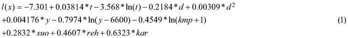
where l(x) = temporary value; t = age (years); d = diameter at breast height (cm); y = latitude in the Uniform Coordinate System (km, here in the range of 6912–6948); kmp = height above sea level (m, here in the range of 91–164); suo = 1 if the plot is located on peatland; reh = 1 if the site type is fertile (OMT or more fertile); kar = 1 if the site type is very poor (Cladina Type or poorer). The results of Eq. 1 were further used to calculate tree level sawlog reductions (Eq. 2).

where si(x) = sawlog reduction, l(x) is the outcome of Eq. 1 and εi = error. During the field work, age was visually evaluated only at the stand-level, which was used for all the trees in the plot. Terrain height was fetched from the DTM provided by the National Land Survey of Finland (Elevation model 10 m, 04/2018). The value of si(x) is always between 0and 1 and it describes the relative reduction in sawlog volume. The final estimates for the factual tree level sawlog volumes were, therefore, calculated by subtracting the product of si(x) and theoretical sawlog volume from the theoretical sawlog volume. Finally, these tree-level volumes were summed to the plot-level and converted to the hectare level (m3 ha–1). The performance of the sawlog reduction model was also tested at the tree-level to examine our additional aim. This performance evaluation was made by inspecting different subsets of pines (e.g. partly defective pines, flawless pines).
Linear mixed-effects model approach (“LME approach”). Linear mixed-effects models were constructed to predict i) factual sawlog volume (m3 ha–1), ii) theoretical sawlog volume (m3 ha–1), and iii) sawlog reduction (m3 ha–1) at the plot-level. Linear models have been commonly used to predict different forest attributes by means of ALS (Næsset 1997). LME approach was used instead of regular linear models, because our data had hierarchical structure (each stand was composed of four plots). The grouped structure of the data was considered by adding stand specific random intercepts into models. However, the utilisation of the random intercept in the prediction would require local measurements, which would not be available in practice. Therefore, only the fixed parts of the models were used for predicting. Ground truth sawlog reduction needed in the modelling was calculated by subtracting the factual sawlog volume from the theoretical sawlog volume. The effect of site fertility was also tested by employing site type dummy variables as additional predictors. Thus, six different LME models were eventually constructed. These models were then used in three different ways to predict factual sawlog volumes. All the models were constructed in the R statistical computing environment (R Core Team 2016) using the nlme package (Pinheiro et al. 2018). The models were fitted with Restricted Maximum Likelihood (Fahrmeir et al. 2013) and had the form as follows (Eq. 3).
![]()
where Xki is the vector of the fixed predictor variables (i.e. ALS metrics and possible site type dummy variables) for plot i in stand k, β is the vector of the regression coefficients for the fixed effects, uk is the random effect for stand k, and eki is the residual error for plot i in stand k.
The predictor variables were chosen from the set of all derived ALS metrics in a process whereby the least significant predictors were deleted in steps until the p-value of each remaining predictor was < 0.001. After this point, the best combination of 2–3 predictors, in terms of RMSE%, BIAS% and overall homoscedasticity of the residuals, was examined manually. In addition, the leave-one-out cross-validation (LOOCV) was used for all models at the stand-level, which ensured that we always ignored the selected 30 × 30 m stand in turn, and fitted the models with the rest of the data. A square root transformation of the response variable was used with every model, so the bias correction was added to the estimates.
Tree list approach (“TL approach”). We constructed the tree lists that include factual sawlog volumes for the target plots using nearest neighbour (NN) imputation (Packalen and Maltamo 2008). The NN methods have been used in several studies (Packalen and Maltamo 2007; Hudak et al. 2008; Latifi et al. 2010) and in operational projects (Maltamo and Packalen 2014). The benefit of the NN imputation is that it allows the construction of tree lists from the trees of training plots (Temesgen et al. 2003; Packalen and Maltamo 2008). We predicted the tree lists by employing ALS metrics and factual sawlog volumes by tree species as predictor and response variables, respectively. A Most Similar Neighbour (MSN) distance was used as a similarity measure in the NN imputations (see Eq. 1 in Moeur and Stage 1995). The selection of predictor variables was implemented following the algorithm proposed in Packalen et al. (2012), which is based on a heuristic optimization algorithm known as a Simulated Annealing (Kirkpatrick et al. 1983). The aim of the algorithm is to minimize the cost function by solving the NN model repeatedly over a fixed number of times. Here, the minimised cost is the weighted mean RMSE% (see Eq. 5) value over all response variables, i.e. sawlog volume of Scots pine, sawlog volume of Norway spruce, and sawlog volume of deciduous trees. The proportions of theoretical sawlog volume by tree species in the field data were used as weights (0.79 for pine, 0.16 for spruce, and 0.05 for deciduous trees, respectively).
We implemented the NN imputations at the plot-level, and the resulting tree lists were constructed from tree lists of selected neighbours (that also contain factual sawlog volumes) retrieved from the five most similar plots with stand-level LOOCV (k value fixed at 5). The weighting of neighbouring plots was evaluated as an inverse of the MSN distance (Eq. 4)
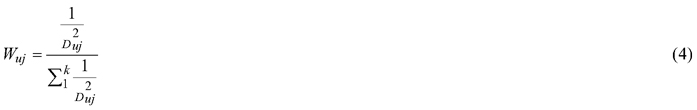
where Wuj is the weight between the plots u (target) and j (reference), k is the number of nearest neighbours and ![]() is the squared MSN distance between plots u and j.
is the squared MSN distance between plots u and j.
2.3.2 Alternatives for the prediction of factual sawlog volumes
The nine alternatives we tested are described below. All of them are applications of previously introduced SRM, LME, or TL approaches. The code in front of the definition (e.g. 2a) will be used henceforth when referring to the alternative in question.
1) Sawlog reduction model was subtracted from the theoretical sawlog volume that was first calculated by taper curves using field measured h, dbh, and d6. The estimated factual sawlog volume was calculated at the tree-level and summed to the plot-level. This alternative does not utilise ALS data and is applied here to show the theoretical level of accuracy that can be obtained without field information on tree quality reductions.
2a) Linear mixed-effects model for factual sawlog volumes.
2b) Alternative 2a + site type considered with additional dummy variables in the LME model.
3a) Linear mixed-effects model for theoretical sawlog volumes subtracted with the SRM.
3b) Alternative 3a + site type considered with additional dummy variables in the LME model.
4a) Linear mixed-effects models for theoretical sawlog volumes and sawlog reduction. The factual sawlog estimate was then calculated by subtracting the latter from the former.
4b) Alternative 4a + site type considered with additional dummy variables in the LME models.
5) Factual sawlog volume imputation using the TL approach.
6) Theoretical sawlog volume imputation from the tree list subtracted with the SRM.
2.4 Accuracy assessment
The modelling was made at the plot-level (15 × 15 m) and the accuracy assessment was made at the stand-level (30 × 30 m), after the plot-level estimates had been first aggregated to the stand-level. Grid level predictions are aggregated to stand level also in operational area-based ALS inventories. We assessed the accuracy of the alternatives at the stand-level using the relative RMSE (Eq. 5) and BIAS (Eq. 6) values.


where n is the number of stands in the dataset,![]() is the observed factual sawlog volume for stand i,
is the observed factual sawlog volume for stand i, ![]() is the predicted factual sawlog volume for stand i and
is the predicted factual sawlog volume for stand i and ![]() is the measured mean of the factual sawlog volume in the dataset. Scatterplots presenting observed vs. predicted values were also examined.
is the measured mean of the factual sawlog volume in the dataset. Scatterplots presenting observed vs. predicted values were also examined.
3 Results
3.1 Linear mixed-effects models
Linear mixed-effects models were built to predict three different attributes: factual sawlog volume, theoretical sawlog volume, and sawlog reduction. In addition, the effect of site fertility was tested by simply adding dummy variables as predictors to the models. The fixed parts, significance of site type dummies, and standard deviations of random effects and residuals of the six models fitted with all data are shown in Table 5. With all models, a greater proportion of the variability not explained by the fixed part was associated with the model error than the random intercepts between stands. Due to square root transformations in the response variables, the right sides of the equations were squared in the prediction phase and a bias correction (standard deviation of random effects + standard deviation of residuals) was also added. RMSE% and BIAS% of the models after LOOCV are also presented in Table 5.
| Table 5. Information of the linear mixed effects models when fitted with all data, excluding the RMSE% and BIAS% values which are after leave-one-out cross-validation. For the fixed parameters, the standard error is given in parentheses. The study area is located in boreal forest in eastern Finland and it is dominated by Scots pine. | ||||||
| LME-1 | LME-2 | LME-3 | LME-4 | LME-5 | LME-6 | |
| Response | (Factual sawlog V)1/2 | (Theoretical sawlog V)1/2 | (Sawlog reduction)1/2 | |||
| Intercept | 9.140 (1.496) | 7.163 (1.492) | 7.379 (1.863) | 5.878 (1.855) | 5.192 (1.109) | 5.317 (1.717) |
| f_h902 | 0.021 (0.001) | 0.021 (0.001) | - | - | - | - |
| l_h90 | - | - | 0.810 (0.050) | 0.804 (0.050) | - | - |
| f_h30 | - | - | - | - | 0.283 (0.063) | 0.283 (0.066) |
| l_d10 | –9.082 (1.663) | –10.008 (1.617) | –14.393 (1.649) | –15.077 (1.646) | - | - |
| f_d2 | - | - | - | - | –8.592 (1.710) | –8.580 (1.790) |
| MT | - | 2.718 (0.772) | - | 2.241 (0.784) | - | –0.124 (1.398) |
| VT | - | 2.843 (0.829) | - | 2.154 (0.841) | - | –0.141 (1.477) |
| var(u) | 0.9742 | 0.8172 | 0.9132 | 0.8162 | 1.5992 | 1.6512 |
| var(e) | 1.2842 | 1.2812 | 1.3312 | 1.3292 | 1.8352 | 1.8362 |
| p(MT) | - | 0.001 | - | 0.007 | - | 0.93 |
| p(VT) | - | 0.002 | - | 0.015 | - | 0.92 |
| RMSE% | 30.85 | 29.46 | 29.18 | 28.18 | 82.45 | 83.27 |
| BIAS% | –0.44 | –0.91 | –0.14 | –0.32 | 3.83 | 3.75 |
| V = volume, f/l denotes whether the metric is derived from the first or last echoes, h30 and h90 are the 30th and 90th height percentiles, d2 and d10 are the densities at heights of 2 and 10 m, MT and VT = site type dummy variables, var = variance, p(MT/VT) = the p-values of corresponding site type dummy variables. | ||||||
3.2 Accuracies associated with factual sawlog volume predictions
The resulting RMSE% values associated with the predicted factual sawlog volume at the stand-level varied from 20.9% to 30.0% (Table 6). The alternative that employed only the LME model for factual sawlog volumes with site type dummy variables (2b) proved to be the most accurate, while the alternative in which the tree list based theoretical sawlog volume was subtracted with SRM (6), was the least accurate. The inclusion of the site type dummy variables into LME models improved the corresponding predictions (2–4). All the alternatives that included SRM (1, 3 and 6) yielded clear overestimates. The LME model based predictions (3) were also more accurate than the theoretical alternative based on actual tree dimensions (alternative 1).
| Table 6. The root mean squared error (RMSE%) and BIAS% values for the predicted factual sawlog volumes with different alternatives at the stand-level (30 × 30 m) in Scots pine dominated boreal forests. Alternatives b always include the site type dummies. See Materials and Methods and Table 5 for detailed definitions. | |||
| Alt. | Definition | RMSE% | BIAS% |
| 1 | Observed theoretical sawlog volume - SRM | 29.08 | –10.26 |
| 2a | LME-1 factual sawlog volume | 22.69 | –0.44 |
| 2b | LME-2 factual sawlog volume | 20.92 | –0.91 |
| 3a | LME-3 theoretical sawlog volume - SRM | 27.16 | –10.19 |
| 3b | LME-4 theoretical sawlog volume - SRM | 25.27 | –10.50 |
| 4a | LME-3 theoretical sawlog volume - LME-5 sawlog reduction | 25.11 | –1.77 |
| 4b | LME-4 theoretical sawlog volume - LME-6 sawlog reduction | 23.78 | –1.98 |
| 5 | TL factual sawlog volume | 27.31 | 3.20 |
| 6 | TL theoretical sawlog volume - SRM | 30.03 | –7.98 |
| Alt. = alternative, LME = linear mixed-effects model, TL = tree list, SRM = sawlog reduction model of Mehtätalo (2002). | |||
In the observed vs. predicted values scatterplots at the stand-level (Fig. 1), only the versions that also included the site type dummies (b) are presented for alternatives 2–4. This was done for the sake of simplicity as the a and b versions were very similar. A general difference can be seen between the alternatives based on the LME models (2–4) and the tree list (5 and 6). Moreover, all three alternatives that included the SRM (1, 3 and 6) also produced overestimates, which is evident in the scatterplots.
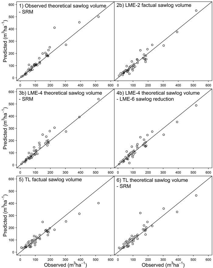
Fig. 1. Observed vs. predicted values for the factual sawlog volume (m3 ha–1) at the stand- level (30 × 30 m). For simplicity, only the b versions of alternatives 2, 3 and 4 are shown. LME = linear mixed-effects model, TL = tree list, SRM = sawlog reduction of Mehtätalo (2002). See Materials and Methods for detailed definitions. The study area is located in boreal forest in eastern Finland and it is dominated by Scots pine.
3.3 Performance of the national sawlog reduction model
We evaluated the performance of the SRM model with different subsets of pines (Table 7). The subset with pines that produced at least one acceptable sawlog (subset 1) resulted in RMSE% values approximately 5% smaller than the subset where all the flawless pines were excluded (subset 2). In addition, this exclusion led to clear overestimates; BIAS% value of subset 2 was –15.3%. However, subset 2 performed considerably better than the subset 4 with the pines that were not flawless. In terms of RMSE% values, the most accurate predictions (30.4%) originated from the subset with only flawless pines (subset 3), although in this case the factual sawlog volume was highly underestimated (BIAS%: 27.8%). The smallest and largest reductions were 15.4% and 63.1%, respectively, which produced standard deviation values three times smaller than the observed value. The BIAS% value was –18% when all pines were included, so the factual sawlog volume, in general, was notably overestimated.
| Table 7. Root mean squared error (RMSE%) and BIAS% values for the model of Mehtätalo (2002) when estimating the factual sawlog volume with different sets of Scots pines. Subset 1 = pines with factual sawlog volume > 0. Subset 2 = pines with factual sawlog volume > 0, but not flawless. Subset 3 = flawless pines. Subset 4 = all defective pines. The main characteristics of the relative sawlog reduction (%) at the tree-level for both observed and modelled values with different sets of pines are also shown. The study area is located in boreal forest in eastern Finland. | ||||||
| RMSE% | BIAS% | MinSR | MaxSR | MeanSR | SdSR | |
| Observed | - | - | 0 | 100 | 39.8 | 36.9 |
| All pines (n = 1235) | 73.6 | –18.0 | 15.4 | 63.1 | 32.4 | 10.4 |
| Subset 1 (n = 971) | 38.8 | 1.3 | 15.4 | 58.5 | 31.2 | 10.0 |
| Subset 2 (n = 625) | 43.7 | –15.3 | 15.4 | 58.5 | 30.1 | 9.6 |
| Subset 3 (n = 346) | 30.4 | 27.8 | 16.1 | 58.2 | 33.3 | 10.2 |
| Subset 4 (n = 889) | 96.9 | –46.7 | 15.4 | 63.1 | 32.1 | 10.5 |
| Sd = standard deviation, SR = sawlog reduction (%). | ||||||
4 Discussion
4.1 Overview of the results and study conditions
Our results imply that under homogenous circumstances, a correlation between ALS metrics and factual sawlog volume exists, although the accuracy of the predictions might not be satisfactory. Also, the accuracy varied considerably between the different alternatives. The alternatives based on LME approach performed better than the alternatives based on TL approach.
While a comparison of our results with previous studies is a challenge due to widely varying conditions and methods, our overall results are in line with previous studies. For example, Bollandsås et al. (2011) predicted the factual sawlog volume at the 50 × 50 m level with a RMSE% value of 24%. At the tree-level, Maltamo et al. (2009) achieved lower RMSE% values with both NN imputation and Seemingly Unrelated Regression methods. However, in addition to a completely different approach, dataset and methods, they also predicted the proportion of sawlogs with respect to stem volume, which is not exactly the same as factual sawlog volume. In general, more studies that consider the prediction of factual sawlog volumes or other quality attributes are needed to distinguish the most applicable approaches and methods.
Our field data only included the factual sawlog volumes for large Scots pines. In addition to pines, the field data also included Norway spruce and birch trees, both of which have high economic value in Finnish forestry. However, as the study was conducted using ABA, other tree species and their factual sawlog volumes could not be just ignored. Therefore, based on the knowledge of strong pine dominance, we also used the theoretical sawlog volume as the factual sawlog volume for these other tree species. In other words, due to data restrictions, we expected that all spruce and birch trees to be flawless (i.e. the sawlog reduction model was not applied to them). In practice, this is obviously not a realistic assumption as different quality requirements apply to spruce- and birch sawlogs as well. This affects the results of alternatives 1, 3, and 6 on mixed-species plots especially, because the factual sawlog volume of spruce and deciduous trees on those plots was assumed to be predicted perfectly. Consequently, SRM had a smaller weighting when total sawlog volumes were predicted. Nevertheless, since the assumption of strong pine dominance holds true (Table 3), the overall effect can be expected to be relatively minor.
4.2 Linear mixed-effects models vs. tree lists
The alternatives based on LME models performed notably better than the TL alternatives (Table 6). There were some general differences between these approaches (described below), so the comparison between alternatives 2 vs. 5, and 3 vs. 6 is not completely straightforward.
Nevertheless, as the TL approach has traditionally performed well in the prediction of other forest attributes (Packalen and Maltamo 2008), the magnitude of the difference related to the predictive performances was surprisingly high in favour of LME approach. Presumably this implies that the training data that was used in the TL method was not comprehensive enough and, therefore, suitable neighbours were not found. In addition, the NN imputation was conducted using three separate response variables (factual sawlog volume of pines, spruce and deciduous trees), and the eventual predictor variables were chosen by minimising the weighted average of the RMSE% values of all response variables. This means that the total factual sawlog volume of all species was not used as a response variable in the NN imputation, but was in the corresponding LME models with a square root transformation (LME-1 and LME-2 in Table 5). An additional minor difference was that alternative 6 was calculated from the same tree list with the species-specific factual sawlog volumes as the response variables, while the response variable in alternative 3 was the square root of total theoretical sawlog volume of all species (LME-3 and LME-4 in Table 5).
We imputed the tree list using a multivariate response configuration that consists of factual sawlog volumes associated with Scots pine, Norway spruce and deciduous species. The multivariate response configuration has been showed to perform well in NN imputation when the MSN distance metric is used (Maltamo and Packalen 2014). The main reason for the selection of the multivariate response was that it ensured that the SRM was only applied to pines. Another reason for the selection of the multivariate response was that the response configuration comprising species-specific attributes is compatible with the operational ALS inventory as implemented in Finland. It is also worth noting that a great advantage of the TL approach is that it also allows (unlike LME models) species separation.
4.3 National tree level sawlog reduction model
All the alternatives that included the sawlog reduction model of Mehtätalo (2002) (1, 3 and 6) yielded clear overestimates (BIAS% –8.0 to –10.5%), which means that quality of pine in the study area is poorer than indicated by the model. This sawlog reduction model is not able to adapt to cases where the whole stem is so defective that quality requirements are not met, even for one sawlog, or where the stem is completely flawless (Table 7). The effects of these two extremes, therefore, compensate each other. Other than that, the RMSE% and BIAS% values varied depending on the set of pines in question. The variation in the main characteristics between subsets was only minor and was not in agreement with the field data, e.g. mean of the relative sawlog reduction was largest with flawless pines (subset 3), although it should have been the smallest. This indicates that the model produces somewhat constant estimates regardless of tree quality. This was also expected, as the main variables in the model are age, diameter at breast height, latitude and the height above sea level, none of which varies notably within our dataset. The dummy variables that consider site type also have a small effect.
The predictions for factual sawlog volumes in alternatives 3 and 6 were obtained by subtracting the SRM from the ALS based theoretical sawlog volume predictions. Therefore, in addition to SRM, the errors in these initial ALS predictions also affected the predictive performance. All the LME models were bias corrected and the tree list based theoretical sawlog volume predictions were almost non-biased (BIAS% was 0.1% and 0.4% with and without site type information, respectively). Consequently, the resulting BIAS% values of alternatives 3a and 3b at the stand-level did not change notably compared to alternative 1, while the BIAS% value of alternative 6 improved by about 2.3% points, respectively. Nevertheless, alternatives 3a and 3b with predicted theoretical sawlog volume at the stand-level yielded smaller RMSE% values than alternative 1 with the observed theoretical sawlog volume, which is somewhat surprising. However, this was not the case at the plot-level prior aggregations (data not shown) as the RMSE% values of alternatives 1, 3a and 3b were 33.0%, 35.9% and 34.4%.
The models of Mehtätalo (2002) were tested also by Malinen et al. (2007), who compared the models with bucking-simulation based approach in the prediction of timber assortment recovery. They reported that in case of pine the sawlog reduction model produced clearly smaller estimates for sawlog recovery than the bucking simulation. This is contradictory to our findings, but comprehensive comparison is again difficult as the datasets originated from different geographical locations, and different methods were used. Nevertheless, the species-specific sawlog reduction models that are presented in Mehtätalo (2002) are in operational use in Finnish forest planning systems (Metsäkeskus 2017). In general, the results in our data were inaccurate, which emphasises the need for more accurate methods to predict factual sawlog volumes locally in operational planning processes.
4.4 Effect of site type
Scots pines are susceptible to branch thickness and crookedness of the stem related defects when they grow on fertile sites. Our field data supports this observation, as both the proportion of fully defective pines and the mean of observed sawlog volume reduction were clearly larger on fertile (OMT) plots than elsewhere (Table 2). The p-values of site type dummy variables were small in LME models for factual and theoretical sawlog volume indicating statistical significance (LME-2 and LME-4 in Table 5). The corresponding large p-values in LME model for sawlog reduction (LME-6 in Table 5) are probably explained by the overall poor performance of the sawlog reduction model (LME-5 in Table 5). Nevertheless, the accuracies of the LME model based alternatives (2–4) clearly improved when site type information was utilised. Therefore, the use of site type information as auxiliary data is probably useful when the aim is to predict the quality associated attributes of Scots pine. For example, in Finnish practical large-scale ALS based forest inventories, site type information might be acquired from the existing stand database, which was collected and updated over decades in the previous inventory method.
5 Conclusions
In general, the factors that cause the reduction in sawlog volumes are difficult to observe from above as they are located in the main stem (possibly also underneath the bark), or in the connection of stem and branches. Additionally, the defects may not show any relationship to crown characteristics. Therefore, the potential for using ALS data to predict commercial tree quality may be limited, because the majority of the laser pulses hit the tree crowns or bare ground instead of the stems. Nevertheless, our results indicate that when an examination is carried out at the 30 × 30 m plot-level under relatively homogenous forest conditions, there is some degree of correlation between the ALS data, and the factual sawlog volume of Scots pine. The best predictive performance (RMSE%: 21%) was obtained with a LME model for the factual sawlog volume. However, the acquisition of the training data with our method is a very laborious task, so a more practical alternative is needed to take account of tree quality attributes in operational ALS inventories.
Acknowledgements
The study was funded by the project “Puuston laatutunnusten mittaus ja mallinnus” of Ministry of Agriculture and Forestry of Finland. We thank the two anonymous reviewers for their constructive comments.
References
Axelsson P. (2000). DEM generation from laser scanner data using Adaptive TIN Models. Proceedings of the XIXth ISPRS Conference, IAPRS, Vol. XXXIII. Amsterdam, The Netherlands. p. 110–117.
Barth A., Möller J.J., Wilhelmsson L., Arlinger J., Hedberg R., Söderman U. (2015). A Swedish case study on the prediction of detailed product recovery from individual stem profiles based on airborne laser scanning. Annals of Forest Science 72(1): 47–56. https://doi.org/10.1007/s13595-014-0400-6.
Bollandsås O.M., Maltamo M., Gobakken T., Lien V., Næsset E. (2011). Prediction of timber quality parameters of forest stands by means of small footprint airborne laser scanner data. International Journal of Forest Engineering 22(1): 14–23. https://doi.org/10.1080/14942119.2011.10702600.
Cajander A.K. (1949). Forest types and their significance. Acta Forestalia Fennica 56(5): 1–71. https://doi.org/10.14214/aff.7396.
Dalponte M., Ene L.T., Gobakken T., Næsset E., Gianelle D. (2018). Predicting selected forest stand characteristics with multispectral ALS data. Remote Sensing 10(4) article 586. https://doi.org/10.3390/rs10040586.
Fahrmeir L., Kneib T., Lang S., Marx B. (2013). Regression models, methods and applications. 1st edition. Springer-Verlag, Berling Heidelberg. 698 p. https://doi.org/10.1007/978-3-642-34333-9_1.
Hauglin M., Hansen E., Sørngård E., Næsset E., Gobakken T. (2018). Utilizing accurately positioned harvester data: Modelling forest volume with airborne laser scanning. Canadian Journal Forest Research 48(8): 913–922. https://doi.org/10.1139/cjfr-2017-0467.
Holmgren J., Barth A., Larsson H., Olsson H. (2012). Prediction of stem attributes by combining airborne laser scanning and measurements from harvesters. Silva Fennica 46(2): 227–239. https://doi.org/10.14214/sf.56.
Hudak A.T., Crookston N.L, Evans J.S., Hall D.E., Falkowski M.J. (2008). Nearest neighbor imputation of species-level, plot-scale forest structure attributes from LiDAR data. Remote Sensing of Environment 112(5): 2232–2245. https://doi.org/10.1016/j.rse.2007.10.009.
Karjalainen T., Korhonen L., Packalen P., Maltamo M. (2019). The transferability of airborne laser scanning based tree level models between different inventory areas. Canadian Journal of Forest Research 49(3): 228–236. https://doi.org/10.1139/cjfr-2018-0128.
Kirkpatrick S., Gelatt C.D., Vecchi M.P. (1983). Optimization by simulated annealing. Science 220(4598): 671–680. https://doi.org/10.1126/science.220.4598.671.
Korhonen L., Peuhkurinen J., Malinen J., Suvanto A., Maltamo M., Packalen P., Kangas J. (2008). The use of airborne laser scanning to estimate sawlog volumes. Forestry 81(4): 499–510. https://doi.org/10.1093/forestry/cpn018.
Laasasenaho J. (1982). Taper curve and volume function for pine, spruce and birch. Communicationes Instituti Forestalis Fenniae 108: 1–74. http://urn.fi/URN:ISBN:951-40-0589-9.
Lämsä P., Kellomäki S., Väisänen H. (1990). Nuorten mäntyjen oksikkuuden riippuvuus puuston rakenteesta ja kasvupaikan viljavuudesta. [Branchiness of young Scots pines as related to stand structure and site fertility]. Folia Forestalia 746: 1–22. http://urn.fi/URN:ISBN:951-40-1092-2.
Latifi H., Nothdurft A., Koch B. (2010). Non-parametric prediction and mapping of standing timber volume and biomass in a temperate forest: applications of multiple optical/LiDAR-derived predictors. Forestry 83(4): 395–407. https://doi.org/10.1093/forestry/cpq022.
Lindroos O., Ringdahl O., La Hera P., Hohnloser P., Hellström T. (2015). Estimating the position of the harvester head – a key step towards the precision forestry of the future? Croatian Journal of Forest Engineering 36(2): 147–164.
Malinen J., Kilpeläinen H., Piira T., Redsven V., Wall T., Nuutinen T. (2007). Comparing model-based approaches with bucking simulation-based approach in the prediction of timber assortment recovery. Forestry 80(3): 309–321. https://doi.org/10.1093/forestry/cpm012.
Maltamo M., Packalen P. (2014). Species-specific management inventory in Finland. In: Maltamo M., Næsset E., Vauhkonen J. (eds.). Forestry applications of airborne laser scanning – concepts and case studies. Managing Forest Ecosystems 27: 241–252. https://doi.org/10.1007/978-94-017-8663-8_12.
Maltamo M., Peuhkurinen J., Malinen J., Vauhkonen J., Packalen P., Tokola T. (2009). Predicting tree attributes and quality characteristics of Scots pine using airborne laser scanning data. Silva Fennica 43(3): 507–521. https://doi.org/10.14214/sf.203.
Mehtätalo L. (2002). Valtakunnalliset puukohtaiset tukkivähennysmallit männylle, kuuselle, koivuille ja haavalle. [Nationwide species-specific sawlog reduction models for Scots pine, Norway spruce, birches and aspen.] Metsätieteen aikakauskirja 4: 575–591. https://doi.org/10.14214/ma.6196.
Metsäkeskus [Finnish Forest Centre]. (2017). Metsään.fi – Your online forest. https://www.metsakeskus.fi/sites/default/files/metsaanfi-eservices-for-forest-owners-broschyr.pdf. [Cited 30 Jan 2019].
Metsäntutkimuslaitos [The Finnish Forest Research Institute]. (2009). Valtakunnan metsien 11. inventointi (VMI 11). Maastotyön ohjeet 2009. Koko Suomi. 2. painos. [11th National Forest Inventory (NFI 11). Field manual for whole Finland. 2nd edition]. 182 p. http://urn.fi/URN:NBN:fi-fe201603038534.
Moeur M., Stage A.R. (1995). Most Similar Neighbor: an improved sampling inference procedure for natural resource planning. Forest Science 41: 337–359.
Næsset E. (1997). Estimating timber volume of forest stands using airborne laser scanner data. Remote Sensing of Environment 61(2): 246–253. https://doi.org/10.1016/S0034-4257(97)00041-2.
Næsset E. (2011). Estimating above-ground biomass in young forests with airborne laser scanning. International Journal of Remote Sensing 32(2): 473–501. https://doi.org/10.1080/01431160903474970.
Packalen P., Maltamo M. (2007). The k-MSN method for the prediction of species-specific stand attributes using airborne laser scanning and aerial photographs. Remote Sensing of Environment 109(3): 328–341. https://doi.org/10.1016/j.rse.2007.01.005.
Packalen P., Maltamo M. (2008). Estimation of species-specific diameter distributions using airborne laser scanning and aerial photographs. Canadian Journal of Forest Research 38(7): 1750–1760. https://doi.org/10.1139/X08-037.
Packalen P., Temesgen H., Maltamo M. (2012). Variable selection strategies for nearest neighbor imputation methods used in remote sensing based forest inventory. Canadian Journal of Remote Sensing 38(5): 557–569. https://doi.org/10.5589/m12-046.
Peuhkurinen J., Maltamo M., Malinen J., Pitkänen J., Packalen P. (2007). Preharvest measurement of marked stands using airborne laser scanning. Forest Science 53(6): 653–661.
Peuhkurinen J., Maltamo M., Malinen J. (2008). Estimating species-specific diameter distributions and saw log recoveries of boreal forests from airborne laser scanning data and aerial photographs: a distribution-based approach. Silva Fennica 42(4): 625–641. https://doi.org/10.14214/sf.237.
Pfennigbauer M., Ullrich A. (2011). Multi-wavelength airborne laser scanning. ILMF 2011, New Orleans. 10 p.
Pinheiro J., Bates D., DebRoy S., Sarkar D., R Core Team. (2018). nlme: linear and nonlinear mixed effects models. R package version 3.1-137. https://CRAN.R-project.org/package=nlme.
R Core Team. (2016). R: a language and environment for statistical computing. R Foundation for Statistical Computing, Vienna, Austria. https://www.R-project.org/.
StanForD. (2012). Standard for forest data and communications. Skogsforsk. https://www.skogforsk.se/contentassets/b063db555a664ff8b515ce121f4a42d1/appendix1_eng_120418.pdf. [Cited 30 Jan 2019].
Temesgen H., LeMay V.M., Froese K.L., Marshall P.L. (2003). Imputing tree-lists from aerial attributes for complex stands of south-eastern British Columbia. Forest Ecology and Management 177(1–3): 277–285. https://doi.org/10.1016/S0378-1127(02)00321-3.
Total of 35 references.
